5.4.7. Structural reliability models and equations

The present paragraph provides limit state functions and guidance for the modelling of several failure mechanisms that are of relevance for mechanical reliability prediction. The content of this paragraph is largely based on [BR_MEC_2], where some aspects are discussed in more detail.

Note

\(G(x)\) is calculated here but to obtain the reliability \(F(x)\) (probability of failures), a method similar to Section 5.4.6.1 needs to be applied.

An overview on the failure mechanisms covered by the different subparagraphs is found in Table 5.4.10. The limit state functions provided in each dedicated subsection are generally applicable with the “full” structural reliability method described in Section 5.4.6.1 and in Part 2 - Methods. Simplified models in the sense of Section 5.4.6.2, with analytic solutions for the probability of failure calculations, are provided for some failure mechanisms. Failure mechanisms that can be modelled with the aid of simple stress strength methods (as discussed in Section 5.4.6.3) are also mentioned in Table 5.4.10, but will not discussed any further in the present paragraph.

Table 5.4.10 Overview on failure mechanisms covered in paragraph 9.7 (see handbook)

Failure mechanism category (cf. Table 5.4.4)	Limit state functions provided in Section 5.4.6	Simplified model?	Paragraphs
Distortion	The modelling of distortion is very case specific, but can often be handled with generic stress strength methods		Section 5.4.6.1,Section 5.4.6.3
Wear	General (adhesive) wear	Yes	Section 5.4.7.1.1
Wear	Solid lubricant wear	Yes	Section 5.4.7.1.2
Wear	Fluid lubricant wear	Yes	Section 5.4.7.1.3
Fracture / Fatigue	High cycle fatigue	Yes	Section 5.4.7.2.1
Fracture / Fatigue	Fatigue crack growth	No	Section 5.4.7.2.2
Fracture / Fatigue	Fracture and low cycle fatigue: stress strength approach		Section 5.4.6.3
Corrosion	Stress corrosion cracking	No	Section 5.4.7.3
Material degradation	Radiation damage	Yes	Section 5.4.7.4.1

Failure mechanisms that are not listed in Table 5.4.10 need to be modelled by the handbook user, possibly making use of published information, e.g. in RiAC’s WARP [NR_MEC_2] or Kowal [BR_MEC_21]. The “full” structural reliability method can be applied with any limit state function or failure mechanism model, see Section 5.4.6.1 for details.

The following subparagraphs dedicated to each failure mechanism model always follow the same logic.

First the failure mechanism is introduced, and a generic limit state function is derived that can be used with general structural reliability methods, possibly requiring numerical methods to derive the probability of failure. Closed form solutions (if available) are then discussed separately under the heading “Simplified failure mechanism model”.

The derivation of these closed-form solutions is based on several assumptions related to the limit state function and the basic variable modelling, see Section 5.4.6.3 for a general introduction. The detailed assumptions are specific to the considered failure mechanisms; a short summary is provided together with each simplified model.

Note

It is not possible to make a general statement how “exact” the analytic solutions are, e.g. when compared to a “full” structural reliability assessment. However, the assumptions listed can and should be checked to decide whether the simplified model can be used for a given application or whether the “full” structural reliability method is more appropriate.

5.4.7.1. Modelling of failures due to mechanical wear

Wear is a complex phenomenon related to the erosion or displacement of material during the contact of solid surfaces. Several types of wear can be distinguished:

• Adhesive wear – displacement and attachment of wear debris from one surface to another,

• Abrasive wear – cutting and deformation of material from a soft surface when a harder surface slides across it (2-body) or due to hard particles between two surfaces (3-body),

• Fretting wear – wear between two solid surfaces experiencing oscillatory relative motion of low amplitude, e.g. induced by vibration,

• Lubricated wear – wear in lubricated contacts,

• Fatigue wear – weakening of a surface by cyclic loading as wear particles are detached by cyclic crack growth of micro-cracks on the surface.

Adhesive, abrasive and fretting wear show common behaviour, and it is commonly agreed that for these types the adhesive wear mechanism plays a dominant role. A general wear model with a focus on adhesive wear is presented in Section 5.4.7.1.1.

Lubricated wear is related to the degradation of the lubricant or the lubricant reservoir in lubricated contacts. This regime is typical for bearings, with analytical models provided in Section 5.4.7.1.2 for solid lubricated bearings (particularly bearing cages), and in Section 5.4.7.1.3 for fluid lubricated bearings.

Finally, fatigue wear is caused by cyclic loading and corresponding crack formation. It is the dominant bearing failure mechanism in on-ground applications, where bearing life is traditionally modelled based on the Lundberg-Palmgren theory [BR_MEC_29] with empirical formulas for the “basic life” of a bearing (corresponding to the number of revolutions at which 10% of the bearings have failed). However, in space applications, bearing lifetime is almost never limited by material fatigue, but instead by the degradation of the lubricant [BR_MEC_16]. For this reason, fatigue wear is not discussed any further in the following.

5.4.7.1.1. Adhesive wear

Adhesive wear is considered as governing for many wear failures and is thus typically used for the analytical prediction of wear. The key parameter for the wear estimation is the volume worn away per unit of sliding distance, which can be estimated based on the classical wear model by Archard [BR_MEC_5], here used in the form of Lancaster [BR_MEC_24].

Failure due to adhesive wear is then modelled with the following limit state function:

Equation

(5.4.17)\[g\left( \text{X}(t) \right) = X_{1} - \Theta \cdot X_{2}(t) = V_{limit} - \Theta \cdot \int_{0}^{T}{K_{H}(t) \cdot S(t) \cdot v(t)\text{d}t}\]

Where, \(V_{limit}\) is the limiting value for the volume worn away, \(\Sigma\) the model uncertainty for the Archard wear model, \(K_{H}\) the specific wear rate, \(S\) the normal load, \(\nu\) the sliding velocity and \(T\) the considered time interval.

As an alternative to the limiting value for the volume worn away, the model can also be reformulated in terms of the wear depth \(d\):

Equation

(5.4.18)\[g\left( \text{X}(t) \right) = X_{1} - \Theta \cdot X_{2}(t) = d_{limit} - \Theta \cdot \int_{0}^{T}{K_{H}(t) \cdot \frac{S(t)}{A_{app}} \cdot v(t)\text{d}t}\]

Where, \(d_{limit}\) is the limiting value for the wear depth \(d\) and \(A_{app}\) is the area of apparent contact. Both limit state functions are basically identical, and either one of them can be used for the wear modelling depending on the problem definition.

By adapting the wear rate, the approach can also be used for other wear mechanisms, such as fretting or abrasive wear. The nature of the wear coefficient is generally very complex and its analytical modelling is difficult. Hence, in practice the Archard model is combined with experimental data, in order to perform lifetime assessments.

Simplified adhesive wear model

Assuming that the specific wear rate \(K_{H}\) is constant over the whole mission (in practice it is typically derived from tests under “worst case” conditions) and that the remaining time dependent variables are constant during certain deterministic time intervals (e.g. different mission phases), the limit state function given in Eq. (5.4.17) can be simplified as follows:

Equation

(5.4.19)\[g\left( \text{X}(t) \right) = X_{1} - \Theta \cdot X_{2}(t) = V_{limit} - \Theta \cdot K_{H} \cdot \sum_{i = 1}^{n_{P}}{P_{i} \cdot t_{i}}\]

Where, \(P_{i} = S_{i} \cdot v_{i}\) corresponds to the sliding work per time unit (the sliding “power”). Thus, \(X_{2}\) is defined as the volume worn away and \(X_{1}\) as the corresponding limiting value.

Detailed variable definitions are given in Table 5.4.11.

Table 5.4.11 Assumed probabilistic models for the simplified adhesive wear model

Variable	Definition of the variable	Unit	Distribution	CoV range
\(V_{limit}\)	Limiting value (worn volume)	[\(\text{m}^{3}\)]	(Lognormal)	\(0 \leq \nu_{V_{limit}} \leq 0.3\)
\(\text{K}_{H}\)	Specific wear rate	[\(\text{Pa}^{-1} = \text{m}^{2}/\text{N}\)]	Lognormal	\(\nu_{\text{K}_{H}} \geq 0\)
\(n_{p}\)	Number of phases / time intervals	[\(-\)]	Deterministic	\(-\)
\(\text{P}_{i}\)	Sliding work / time unit in interval \(i\)	[Nm/s]	Lognormal	\(\nu_{\text{P}_{i}} \geq 0\)
\(\text{t}_{i}\)	Length of time interval \(i\)	[s]	Deterministic	\(-\)
\(\Theta\)	Model uncertainty	[\(-\)]	Lognormal	\(\nu_{\Theta} = 0.2\)

The expected values and coefficients of variation of and are determined as follows:

The expected values and coefficients of variation of \(X_{1}\) and \(X_{2}\) are determined as follows:

Equation

(5.4.20)\[\mu_{X_{1}} = \text{E}\lbrack V_{limit}\rbrack\]

Equation

(5.4.21)\[\mu_{X_{2}} = \text{E}\left\lbrack K_{H} \right\rbrack \cdot \sum_{i = 1}^{n_{P}}{\text{E}\left\lbrack P_{i} \right\rbrack \cdot t_{i}}\]

Equation

(5.4.22)\[\nu_{X_{1}} = \nu_{V_{limit}} = \frac{\sqrt{\text{Var}\lbrack V_{limit}\rbrack}}{\text{E}\lbrack V_{limit}\rbrack}\]

Equation

(5.4.23)\[\nu_{X_{2}} = \sqrt{\nu_{K_{H}}^{2} + \left( 1 + \nu_{K_{H}}^{2} \right) \cdot \frac{\text{Var}\left\lbrack \sum_{i = 1}^{n_{P}}{P_{i} \cdot t_{i}} \right\rbrack}{\left( \sum_{i = 1}^{n_{P}}{\text{E}\left\lbrack P_{i} \right\rbrack \cdot t_{i}} \right)^{2}}}\]

Equation

(5.4.24)\[ \begin{align}\begin{aligned}\text{Var}\left\lbrack \sum_{i = 1}^{n_{P}}{P_{i} \cdot t_{i}} \right\rbrack = \sum_{i = 1}^{n_{P}}{\text{Var}\left\lbrack P_{i} \right\rbrack \cdot t_{i}^{2}} + 2\sum_{i = 1}^{n_{P}}{\sum_{j = i + 1}^{n_{P}}{\text{Cov}\left\lbrack P_{i},P_{j} \right\rbrack \cdot t_{i} \cdot t_{j}}} =\\ \sum_{i = 1}^{n_{P}}{\text{Var}\left\lbrack P_{i} \right\rbrack \cdot t_{i}^{2}} + 2\sum_{i = 1}^{n_{P}}{\sum_{j = i + 1}^{n_{P}}{\rho_{P_{i}P_{j}} \cdot \sqrt{\text{Var}\left\lbrack P_{i} \right\rbrack \cdot \text{Var}\left\lbrack P_{j} \right\rbrack} \cdot t_{i} \cdot t_{j}}}\end{aligned}\end{align} \]

Where, \(\rho_{P_{i}P_{j}}\) denotes the correlation between the sliding work per time unit in different mission phases. The correlation structure can be defined in a simplified way, e.g. assuming \(\rho_{P_{i}P_{j}} = 1\) if the sources of uncertainty in \(P\) are the same in mission phase \(i\) and \(j\) and \(\rho_{P_{i}P_{j}} = 0\) if thereare different uncertainty sources. Assuming full correlation increases the coefficient of variation of \(X_{2}\), which is conservative for small probabilities of failure.

The approach can be further simplified when considering only one mission phase (i.e. \(n_{P} = 1\)), leading to:

\(\text{Var}\left\lbrack \sum_{i = 1}^{n_{P}}{P_{i} \cdot t_{i}} \right\rbrack = \text{Var}\lbrack P\rbrack \cdot t^{2}\).

In practice, this can also be used as a conservative simplification for \(n_{P} > 1\), taking \(P\) from the most critical phase and \(t\) as the total length of the mission. Another strong simplification is possible if the uncertainty in the sliding work per time unit is negligibly small. In this case, the uncertainty in the sum can be neglected and the variance term in Eq. (5.4.24) becomes zero.

With the distributional assumptions in Table 5.4.11, an analytic solution for the probability of failure calculations is derived based on a Lognormal approximation for \(X_{2}\):

Equation

(5.4.25)\[P_{f} (t) = P[X_{1} - X_{2}(t) \cdot \Theta \leq 0] = \text{Φ}\left( \frac{\text{ln}\left(\text{E}\lbrack\Theta\rbrack \right) - \text{ln}\left(\frac{\mu_{X_{1}}}{\mu_{X_{2}}} \right) + 0.5\left( \text{ln}\left(v_{X_{1}}^{2} + 1 \right) - \text{ln}\left( v_{X_{2}}^{2} + 1 \right) -\text{ln}\left( v_{\Theta}^{2} + 1 \right)\right)}{\sqrt{\text{ln}\left( v_{X_{1}}^{2} + 1 \right)\text{+ln}\left(v_{X_{2}}^{2} + 1 \right)\text{+ln}\left( v_{\Theta}^{2} + 1 \right)}}\right)\]

The main assumptions underlying the simplified adhesive wear model are summarized as follows:

• The mission - or the considered time interval \(t\) - is divided into \(n_{P}\) intervals with known (deterministic) duration \(t_{i}\).

• The wear rate \(K_{H}\) is constant over the whole mission (all time intervals \(i\)).

• The normal load \(S_{i}\) and sliding velocity \(v_{i}\) (or the sliding work per time unit \(P_{i} = S_{i} \cdot v_{i}\)) are constant during each time interval \(t_{i}\).

• The distributions of all basic variables can be represented by the models listed in Table 5.4.11. Other models for \(K_{H}\) and \(P_{i}\) are possible as long as the distribution of \(X_{2}\) can still be approximated by a Lognormal distribution.

• The effect of the lognormal assumption for \(X_{1} = V_{limit}\) has been investigated in [BR_MEC_2]. It can lead to an underestimation of the probability of failure, see Fig. 5.4.6 below.

Due to the effect of the last assumption, the analytic method should not be used without justification if the coefficient of variation of \(X_{1} = V_{limit}\) is larger than \(0.3\).

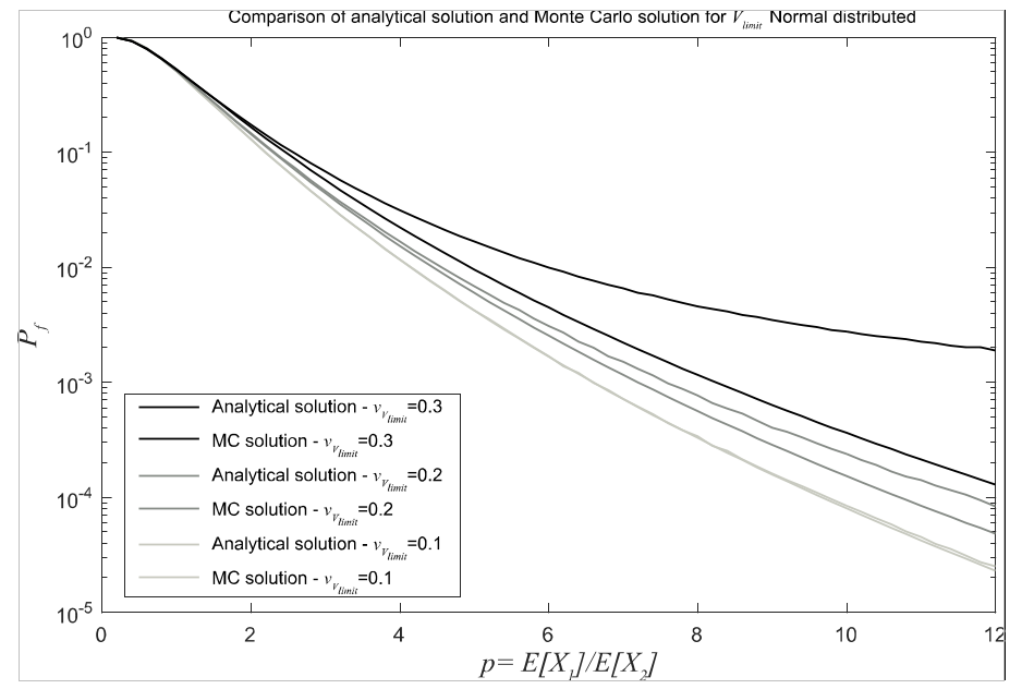
Fig. 5.4.6 Comparison of the analytic solution in Eq. (5.4.26) (adhesive wear model with lognormal distributed* \(V_{limit}\)) with Monte Carlo results for Normal distributed \(V_{limit}\)

5.4.7.1.2. Solid lubricant wear

Due to the fact that solid lubricants do not evaporate, they are suitable for extreme temperatures (both cold and hot) and for applications where contamination could be an issue, e.g. in optical systems. In order to enable on-ground testing and to support the lubrication regime during operations, the lubricant (e.g. sputtered MoS₂) ) is stored in special reservoirs such as cages in case of bearings, which are at the same time used to avoid ball collisions in ball bearings. When the lubricant is degraded, new lubricant is provided via the wear of the reservoir.

In the following, solid lubricant wear modelling is described taking example in a ball bearing. The modelling is applicable to other cases of solid lubricant wear; however, the number of revolutions should be substituted with another suitable measure of sliding distance.

The modelling easily can be adapted from the adhesive wear model given in Section 5.4.7.1. Wear is realized during cage/ball contact; hence the relation \(\int_{0}^{t}{S(t) \cdot v(t)\text{d}t}\) in Eq. (5.4.17) or Eq. (5.4.18) represents the work of the ball/cage interaction forces.

For the bearing example, time is replaced by the number of revolutions \(rev\). The quality \(\int_{0}^{t}{S(t) \cdot v(t)\text{d}t} = \int_{0}^{rev}{\alpha(rev)\text{d}rev}\) can be used for experimental evaluation of the average ball/cage interaction forces, defining a new interaction parameter \(\alpha\).

Simplified solid lubricant wear model

Go to model

Using the simplified form of the adhesive wear model in Eq. (5.4.19) (assuming constant conditions during each mission phase), a limit state function for solid lubricant wear can be derived as follows:

Equation

(5.4.26)\[g\left( \text{X}(t) \right) = X_{1} - \Theta \cdot X_{2}(t) = V_{limit} - \Theta \cdot \sum_{i = 1}^{n_{P}}{K_{H,i} \cdot \alpha_{i} \cdot {rev}_{i}}\]

Where, \(X_{2}\) is defined as the volume worn away and \(X_{1}\) as the corresponding limiting value. Detailed variable definitions are given in Table 5.4.12.

It should be noted that the parameter \(\alpha_{i}\), defined as the average work of ball/cage interaction forces per bearing revolution, will typically be estimated from tests and is thus dependent on the wear rate \(K_{H,i}\). This is the reason why the wear rate cannot easily be taken out of the sum, as in Eq. (5.4.19) for the general adhesive wear model.

Table 5.4.12 Assumed probabilistic models for the simplified solid lubricant wear model

Variable	Definition of the variable	Unit	Distribution	CoV range
\(V_{limit}\)	Limiting value (worn volume)	[\(\text{m}^{3}\)]	(Lognormal)	\(0 \leq \nu_{V_{limit}} \leq 0.3\)
\(\text{K}_{H,i}\)	Specific wear rate in interval \(i\)	[\(\text{Pa}^{-1} = \text{m}^{2}/\text{N}\)]	Lognormal	\(\nu_{\text{K}_{H,i}} \geq 0\)
\(n_{p}\)	Number of phases / time intervals	[\(-\)]	Deterministic	\(-\)
\(\alpha_{i}\)	Ball-cage interaction in interval \(i\)	[Nm]	Lognormal	\(\nu_{\alpha_{i}} \geq 0\)
\(\text{rev}_{i}\)	Number of revolutions in interval \(i\)	[\(-\)]	Deterministic	\(-\)
\(\Theta\)	Model uncertainty	[\(-\)]	Lognormal	\(\nu_{\Theta} = 0.2\)

The expected values and coefficients of variation of \(X_{1}\) and \(X_{2}\) are determined as follows:

Equation

(5.4.27)\[\mu_{X_{1}} = \text{E}\lbrack V_{limit}\rbrack\]

Equation

(5.4.28)\[\mu_{X_{2}} = \sum_{i = 1}^{n_{P}}{\text{E}\left\lbrack K_{H,i} \cdot \alpha_{i} \right\rbrack \cdot {rev}_{i}} = \sum_{i = 1}^{n_{P}}{\left( \text{E}\left\lbrack K_{H,i} \right\rbrack \cdot \text{E}\left\lbrack \alpha_{i} \right\rbrack + \text{Cov}\left\lbrack K_{H,i},\alpha_{i} \right\rbrack \right) \cdot {rev}_{i}}\]

Equation

(5.4.29)\[v_{X_{1}} = v_{V_{limit}} = \frac{\sqrt{\text{Var}\lbrack V_{limit}\rbrack}}{\text{E}\lbrack V_{limit}\rbrack}\]

Equation

(5.4.30)\[v_{X_{2}} = \frac{1}{\mu_{X_{2}}}\sqrt{\sum_{i = 1}^{n_{P}}{\text{Var}\left\lbrack K_{H,i}\alpha_{i} \right\rbrack \cdot {rev}_{i}^{2}} + 2\sum_{i = 1}^{n_{P}}{\sum_{j = i + 1}^{n_{P}}{\text{Cov}\left\lbrack K_{H,i}\alpha_{i},K_{H,j}\alpha_{j} \right\rbrack \cdot {rev}_{i} \cdot {rev}_{j}}}}\]

Assuming full correlation to derive the covariance between \(K_{H,i}\) and \(\alpha_{i}\) (for Eq. (5.4.28)) and for the product of the two variables between different time intervals (for Eq. (5.4.28)) leads to conservative results. As in the general adhesive wear model, the problem can be simplified by considering only one mission phase (\(n_{P} = 1\)), requiring assumptions only on the covariance in Eq. (5.4.28); the covariance term in Eq. (5.4.28) can be dropped if \(n_{P} = 1\).

With the distributional assumptions in Table 5.4.12, an analytic solution for the probability of failure is derived based on a lognormal approximation for \(X_{2}\):

Equation

(5.4.31)\[P_{f} (t) = P[X_{1} - X_{2}(t) \cdot \Theta \leq 0] = \text{Φ}\left( \frac{\text{ln}\left( \text{E}\lbrack\Theta\rbrack \right) - \text{ln}\left( \frac{\mu_{X_{1}}}{\mu_{X_{2}}} \right) + 0.5\left( \text{ln}\left( v_{X_{1}}^{2} + 1 \right) - \text{ln}\left( v_{X_{2}}^{2} + 1 \right) - \text{ln}\left( v_{\Theta}^{2} + 1 \right) \right)}{\sqrt{\text{ln}\left( v_{X_{1}}^{2} + 1 \right)\text{+ln}\left( v_{X_{2}}^{2} + 1 \right)\text{+ln}\left( v_{\Theta}^{2} + 1 \right)}} \right)\]

The main assumptions underlying the simplified solid lubricant wear model are the following:

• The mission is divided into \(n_{P}\) intervals with known number of revolutions \({rev}_{i}\),

• The wear rate \(K_{H,i}\) and ball-cage interaction work \(\alpha_{i}\) are constant during each interval,

• The distributions of all basic variables can be represented by the models listed in Table 5.4.12. Other models for \(K_{H,i}\) and \(\alpha_{i}\) are possible as long as the distribution of \(X_{2}\) can still be approximated by a Lognormal distribution,

• The effect of the Lognormal assumption for \(X_{1} = V_{limit}\) can lead to an underestimation of the probability of failure, see [BR_MEC_2] and Fig. 5.4.6.

Due to the effect of the last assumption, the analytic method should not be used without justification if the coefficient of variation of \(X_{1} = V_{limit}\) is larger than 0.3.

5.4.7.1.3. Fluid lubricant wear

In this paragraph a fluid lubricant wear modelling is described taking example in a ball bearing again. The modelling is applicable to other cases of fluid lubricant wear, but the number of revolutions has to be substituted with another measure of sliding distance in this case.

The starting point for the modelling of fluid lubricant wear is the following limit state function, see [BR_MEC_28] for details:

Equation

(5.4.32)\[g\left( \text{X}(t) \right) = X_{1} - \Theta \cdot X_{2}(t) = M_{0} - M_{inactive} - \Theta \cdot \frac{\frac{N_{b}}{2} \cdot \left( 1 - \frac{b_{d}}{p_{d}} \cdot \cos\vartheta \right)}{2 \cdot K \cdot \exp\left( - 3.35p_{m} \right)} \cdot rev(t)\]

Where, \(M_{0}\) denotes the initial mass of the lubricant, \(M_{inactive}\) the mass of lubricant not participating in the contact (e.g. due to evaporation), and \(\Theta\) the model uncertainty for the associated term, which represents the model to estimate lubricant life described in [BR_MEC_28]. In this term, \(N_{b}\) denotes the number of balls in the bearing, \(p_{d}\) the pitch diameter, \(b_{d}\) the ball diameter, \(\vartheta\) the contact angle, \(K\) is an empirical constant, \(p_{m}\) the contact pressure and \(rev\) the number of revoluations during the considered time interval \(t\).

The variables related to bearing geometry are illustrated in the figure given below.

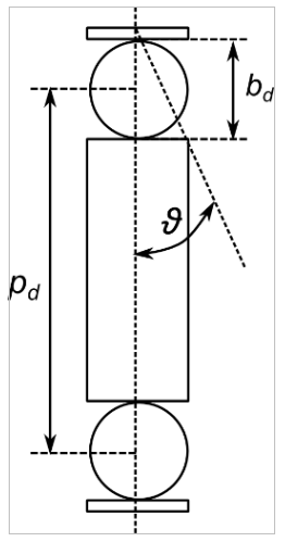
Fig. 5.4.7 Bearing geometry

Simplified fluid lubricant wear model

Go to model

For the simplified modelling, it is considered sufficient to model only \(\Theta\) and \(K\) as random variables; all other variables in Eq. (5.4.32) are assumed to be deterministic. Since the relation for the bearing life from [BR_MEC_28], \(K \cdot \text{exp}\left( - 3.35 \cdot p_{m} \right)\), is purely empirical, curve fitting residuals or the distribution of the coefficient \(K\) can be used for the probabilistic assessments.

Note that in principle, \(M_{inactive}\) can also be treated as stochastic, but its value will generally be only a small fraction of \(M_{0}\), typically not exceeding 1-2% when considering only evaporation losses for a bearing with a labyrinth seal under optimal temperature conditions [BR_MEC_28].

It is furthermore assumed that all variables (except for the number of revolutions \(rev\)) are constant over the whole length of the mission. \(M_{inactive}\) should be estimated considering the amount of lubricant that has evaporated (or is not participating in the contact due to other reasons) at the end of the mission. In reality the amount of evaporated lubricant depends on the number of revolutions, thus the proposed approach leads to a slightly conservative estimation.

These assumptions allow the application of Eq. (5.4.32) without any further simplifications in the limit state function. Thus, \(X_{1} = M_{0} - M_{inactive}\) is defined as the amout of lubricant available and \(X_{2}\) as the amount of lubricant required for the mission, estimated based on the lubricant life model presented in [BR_MEC_28]. Detailed variable definitions are reminded in Table 5.4.13 below.

Table 5.4.13 Assumed probabilistic models for the simplified fluid lubricant wear model

Name	Description	Unit	Type	Cov range
\(M_0\)	Initial mass of the lubricant in the bearing	\(g\)	deterministic	\(-\)
\(M_{\text{inactive}}\)	Mass of lubricant not participating in the contact (e.g. due to evaporation)	\(g\)	deterministic	\(-\)
\(K\)	Empirical constant of the lubricant life model	\(-\)	Lognormal	\(\nu_{K} > 0\)
\(N_b\)	Number of balls in the bearing	\(-\)	deterministic	\(-\)
\(p_d\)	Pitch diameter	\(m\)	deterministic	\(-\)
\(b_d\)	Ball diameter	\(m\)	deterministic	\(-\)
\(\vartheta\)	Contact angle	\(rad\)	deterministic	\(-\)
\(p_m\)	Contact pressure	\(GPa\)	deterministic	\(-\)
\(r\)	Number of revolutions	\(-\)	deterministic	\(-\)
\(\Theta\)	Model uncertainty	\(-\)	Lognormal	\(\nu_{\Theta} = 0.2\)

The mean value of \(X_{1}\) is determined as \(\mu_{X_{1}} = M_{0} - M_{inactive}\) with coefficient of variation \(v_{X_{1}} = 0\). For \(X_{2}\), the following equations can be used:

Equation

(5.4.33)\[\mu_{X_{2}} = \frac{\left( v_{K}^{2} + 1 \right)}{\text{E}\lbrack K\rbrack} \cdot \frac{\frac{N_{b}}{2} \cdot \left( 1 - \frac{b_{d}}{p_{d}} \cdot \cos\vartheta \right)}{2 \cdot \exp\left( - 3.35p_{m} \right)} \cdot rev\]

Equation

(5.4.34)\[v_{X_{2}} = v_{K} = \frac{\sqrt{\text{Var}\lbrack K\rbrack}}{\text{E}\lbrack K\rbrack}\]

The probability of failure is estimated as follows:

Equation

(5.4.35)\[P_{f} (t) = P[X_{1} - X_{2}(t) \cdot \Theta \leq 0] = \text{Φ}\left( \frac{\text{ln}\left( \text{E}\lbrack\Theta\rbrack \right) - \text{ln}\left( \frac{\mu_{X_{1}}}{\mu_{X_{2}}} \right) - 0.5\left( \text{ln}\left( v_{X_{2}}^{2} + 1 \right) + \text{ln}\left( v_{\Theta}^{2} + 1 \right) \right)}{\sqrt{\text{ln}\left( v_{X_{2}}^{2} + 1 \right)\text{+ln}\left( v_{\Theta}^{2} + 1 \right)}} \right)\]

The main assumptions underlying the simplified fluid lubricant wear model are the following:

• Failures in fluid lubricant wear are dominated by the life of the lubricant.

• The amount of lubricant not participating in the contact (e.g. due to evaporation), \(M_{inactive}\), is a small fraction of the initial amount of lubricant, \(M_{0}\) (1-2% for bearings with a labyrinth seal under optimal temperature condition).

• The estimate for the (deterministic) variable \(M_{inactive}\) is chosen conservatively, e.g. by determining the amount of lubricant evaporated at the end of the mission based on the model provided in [BR_MEC_28].

• The uncertainty in most of the variables listed in Table 5.4.13 (except for the empirical constant of the lubricant life model \(K\) and the model uncertainty \(\Theta\)) can be neglected.

• The distributions of \(K\) and \(\Theta\) can be represented by the models listed in Table 5.4.13.

5.4.7.2. Modelling of failures due to fatigue

Fatigue is a failure mechanism incurred by cyclic loading, leading to the initiation and extension of cracks, which degrade the strength of materials and structures.

Failures due to fatigue can be considered as the consequence of several steps:

1. Formation of the crack (crack initiation),

2. Small-crack growth,

3. Large-crack growth,

4. Failure by fracture.

Two loading conditions are distinguished:

• High-cycle fatigue: A high-frequency, low-amplitude loading condition created by structural, acoustic, or aerodynamic vibrations that can propagate flaws to failure.

• Low-cycle fatigue: A low-frequency, high-amplitude loading condition created by thermal, pressure, or structural loads that can propagate flaws to failure.

Failures due to low-cycle fatigue are driven by accumulated plastic deformations, which are typically not allowed (i.e. the design is restricted to elastic regime). If necessary, low-cycle fatigue can be assessed by the ultimate failure criterion, e.g. by means of non-linear finite element analysis with dedicated failure models or dedicated criteria like Manson-Coffin failure criterion. The probability of failure can be assessed using general structural reliability or stress strength methods.

1. The Wöhler provides the degradation of the safety factor as a function of the number of cycles,

2. The Basquin law may provide efficient support to model fatigue phenomena based on experimental data (issued from stress / fatigue test for example).

In the remainder of this section, only high-cycle fatigue is considered.

The standard approach to the fracture control for space projects is presented in [BR_MEC_14]. Depending on the criticality, different approaches can be used:

• Fail safe – damage tolerance design principle, where a structure has redundancy to ensure that failure of one structural element does not cause general failure of the entire structure during the remaining lifetime.

• Safe life – fracture-control design principle, for which the largest undetected defect that can exist in the part does not grow to failure when subjected to the cyclic and sustained loads and environments encountered during the lifetime.

• Low risk of fracture – e.g. when the stress level is below the endurance limit \(C\), then assessment can be performed approximately based on stress and endurance limit only.

Crack formation analysis is typically performed for the fail-safe approach, in order to ensure that failure of one redundant structural element does not cause general failure of the entire structure during the remaining lifetime. This analysis is performed based on the S/N curve approach, whose application for reliability modelling is outlined in Section 5.4.7.2.1.

The safe life principle implies an assessment of the crack growth using fatigue crack growth models, as discussed in Section 5.4.7.2.2. Environmental properties can also be considered in these models, allowing the consideration of failure mechanisms due to stress corrosion cracking (SCC).

5.4.7.2.1. High cycle fatigue modelling with the S/N curve approach

Crack generation due to high cycle fatigue is most commonly modelled using so-called S/N curves relating a stress level or equivalent stress \(S_{eq}\) to the number of cycles to failure, \(N_{f}\):

Equation

(5.4.36)\[\text{log}_{10}\left( N_{f} \right) = A - B \cdot \text{log}_{10}\left( S_{eq} - C \right)\]

Where, the equivalent stress is determined as follows:

Equation

(5.4.37)\[S_{eq} = S_{\max}(1 - R)^{P} = S_{\max}\left( 1 - \frac{S_{\min}}{S_{\max}} \right)^{P}\]

Where, \(S_{\min}\) and \(S_{\max}\) denoting the minimum and maximum stress during one load cycle and \(A\), \(B\), \(C\) and \(P\) are model parameters of the S/N curve model that can be derived from test data, e.g. those presented in [BR_MEC_27] or its predecessor,[BR_MEC_23]. Of special interest is the parameter \(C\), corresponding to the fatigue limit stress, or endurance limit, under which it is assumed that no fatigue failure occurs, thus \(N_{f}(S \leq C) \rightarrow \infty\).

The S/N curve is valid for cyclic loading with constant amplitude or equivalent stress. For cyclic loading with varying stress levels, the S/N curve is combined with the Palmgren-Miner accumulation law to estimate the accumulated damage \(D_{tot}\) after \(N\) stress cycles:

Equation

(5.4.38)\[ \begin{align}\begin{aligned}D_{tot} = \sum_{i = 1}^{N}\frac{1}{N_{f,i}} = \sum_{i = 1}^{N}{10^{- A} \cdot \left( \text{max}\left\lbrack S_{eq,i} - C;0 \right\rbrack \right)^{B}}\\= \ \sum_{j = 1}^{k}{N_{j} \cdot 10^{- A} \cdot \left( \text{max}\left\lbrack S_{eq,j} - C;0 \right\rbrack \right)^{B}}\end{aligned}\end{align} \]

Where, each \(S_{eq,i}\) is drawn from the distribution of equivalent stresses derived from the loading process. The second line in Eq. (5.4.38) is derived by dividing the continuous distribution of \(S_{eq,i}\) into a discrete number of bins. In this final expression, \(k\) denotes the number of bins, \(N_{j}\) the number of cycles in each bin and \(S_{eq,j}\) the corresponding equivalent stress representative for each bin.

As a failure criterion, the accumulated damage \(D_{tot}\) is compared with a fixed threshold \(D_{cr}\) that is typically assumed to be equal to one. However, due to the empirical nature of Miner’s law, failures can also occur at values for \(D_{tot}\) that are below or above unity and \(D_{cr}\) should be considered as a random variable.

A limit state function for high-cycle fatigue is now derived as follows:

Equation

(5.4.39)\[ \begin{align}\begin{aligned}g\left(X(t)\right) = X_{1} - \Theta \cdot X_{2} = D_{cr} - \Theta \cdot D_{tot}\\D_{cr} - \Theta \cdot \sum_{i = 1}^{N(t)}{10^{- A} \cdot \left( \text{max}\left\lbrack S_{eq,i} - C;0 \right\rbrack \right)^{B}}\\= D_{cr} - \Theta \cdot \sum_{j = 1}^{k}{N_{j}(t) \cdot 10^{- A} \cdot \left( \text{max}\left\lbrack S_{eq,j} - C;0 \right\rbrack \right)^{B}}\end{aligned}\end{align} \]

Note

The time dependent formulation in Eq. (5.4.39) neglects load history effects, which is consistent with the accumulative nature of the Palmgren-Miner model. However, when the goal is to evaluate the probability of failure in different mission phases, the accumulated damage contribution of each load event (e.g. testing, launch, in-orbit) should be evaluated separately.

Simplified S/N curve modelling

Go to model

The starting point for the simplified model is the limit state function in Eq. (5.4.39), with load cycles summarized in bins (last row). For the simplified approach, the variables \(N_{j}\), \(B\) and \(C\) are assumed to be deterministic. The uncertainty associated with the loading \(S_{eq,j}\) is then the only uncertainty that cannot be taken out of the sum. A simple approach to model this uncertainty is to multiply deterministic values for \(S_{eq,j}\) (e.g. taken from design calculations) with a random stress scaling factor \(SSF\) that is applied globally, i.e. taking on the same value for all bins [BR_MEC_26]. If it is furthermore assumed that the endurance limit \(C\) equals zero (which is conservative for all applications), the limit state function defined in Eq. (5.4.39) can be brought into the following simple expression:

Equation

(5.4.40)\[g\left( \mathbf{X}(t) \right) = X_{1} - \Theta \cdot X_{2} = D_{cr} - \Theta \cdot D_{tot} = D_{cr} - \Theta \cdot 10^{- A} \cdot {SSF}^{B} \cdot \sum_{j = 1}^{k}{N_{j} \cdot {S_{eq,j}}^{B}}\]

Thus, \(X_{2}\) is defined as accumulated damage, which is calculated based on the S/N curve approach with the Palmgren-Miner accumulation law, and \(X_{1}\) as the corresponding limiting value. Detailed variable definitions are reminded in Table 5.4.14 .

Table 5.4.14 Assumed probabilistic models for the simplified high-cycle fatigue model

Variable	Definition of the variable	Unit	Distribution	CoV range
\(D_{cr}\)	Threshold for accumulated damage	\([-]\)	Lognormal	\(\nu_{D_{cr}} \geq 0\)
\(A\)	S/N curve slope	\(\log(N/m^2)^{-1}\)	Normal	\(\nu_{A} \geq 0\)
\(B\)	S/N curve intercept	\([-]\)	deterministic	\(-\)
SSF	Global stress scaling factor	\([-]\)	Lognormal	\(\nu_{\text{SSF}} \geq 0\)
\(k\)	Number of bins / load events	\([-]\)	deterministic	\(-\)
\(S_{eq,j}\)	(Equivalent) stress in load event \(j\)	\(N/m^2\)	deterministic	\(-\)
\(N_{j}\)	(Equivalent) number of cycles in load event \(j\)	\([-]\)	deterministic	\(-\)
\(\Theta\)	Model uncertainty	\([-]\)	Lognormal	\(\nu_{\Theta} \geq 0\)

Without additional information, the expected value of \(D_{cr}\) can be assumed to be equal to unity and its coefficient of variation equal to 0.3 (based on JCSS [BR_MEC_20] and Wirsching [BR_MEC_33]). The mean value and coefficient of variation of the stress scaling factor \(SSF\) can be determined as follows.

First an appropriate coefficient of variation \(v_{SSF}\) reflecting all uncertainties associated with the load analysis is chosen, considering the most uncertain load event to be conservative. The mean value of the stress scaling factor then depends on the definition of the \(S_{eq,j}\) values. Design values for fatigue stresses are typically defined as upper fractile values, leading to the following relationship:

Equation

(5.4.41)\[\text{E}\lbrack SSF\rbrack = \frac{\sqrt{v_{SSF}^{2} + 1}}{\text{exp}\left( \Phi^{- 1}(\alpha) \cdot \sqrt{\text{ln}\left( v_{SSF}^{2} + 1 \right)} \right)}\]

Where, \(\Phi^{- 1}( \cdot )\) denotes the inverse of the Standard Normal distribution function and \(\alpha\) is the probability that the stresses will be smaller than \(S_{eq,j}\).

Finally, the expected values and coefficients of variation of \(X_{1}\) and \(X_{2}\) are determined as follows:

Equation

(5.4.42)\[\mu_{X_{1}} = \text{E}\lbrack D_{cr}\rbrack\]

Equation

(5.4.43)\[\mu_{X_{2}} = \text{E}\left\lbrack 10^{- A} \cdot {SSF}^{B} \right\rbrack \cdot \sum_{j = 1}^{k}{N_{j} \cdot S_{eq,j}^{B}}\]

Equation

(5.4.44)\[\text{E}\left\lbrack 10^{- A} \cdot {SSF}^{B} \right\rbrack = 10^{- E\lbrack A\rbrack + \frac{1}{2}\text{∙ln}(10) \cdot Var\lbrack A\rbrack} \cdot {E\lbrack SSF\rbrack}^{B} \cdot \left( \sqrt{v_{SSF}^{2} + 1} \right)^{B^{2} - B}\]

Equation

(5.4.45)\[v_{X_{1}} = v_{D_{cr}} = \frac{\sqrt{\text{Var}\lbrack D_{cr}\rbrack}}{\text{E}\lbrack D_{cr}\rbrack}\]

Equation

(5.4.46)\[v_{X_{2}} = \sqrt{10^{Var\lbrack A\rbrack\text{∙ln}(10)} \cdot \left( \sqrt{v_{SSF}^{2} + 1} \right)^{B^{2}} - 1}\]

With the distributional assumptions in Table 5.4.14, an analytic solution for the probability of failure calculations is derived as follows:

Equation

(5.4.47)\[ \begin{align}\begin{aligned}P_{f} (t) = P[X_{1} - X_{2}(t) \cdot \Theta \leq 0]\\= \text{Φ}\left( \frac{\text{ln}\left( \text{E}\lbrack\Theta\rbrack \right) - \text{ln}\left( \frac{\mu_{X_{1}}}{\mu_{X_{2}}} \right) + 0.5\left( \text{ln}\left( v_{X_{1}}^{2} + 1 \right) - \text{ln}\left( v_{X_{2}}^{2} + 1 \right) - \text{ln}\left( v_{\Theta}^{2} + 1 \right) \right)}{\sqrt{\text{ln}\left( v_{X_{1}}^{2} + 1 \right)\text{+ln}\left( v_{X_{2}}^{2} + 1 \right)\text{+ln}\left( v_{\Theta}^{2} + 1 \right)}} \right)\end{aligned}\end{align} \]

With large coefficients of variation for the S/N curve parameter \(A\) and/or the stress scaling factor \(SSF\), both \(v_{X_{2}}\) and \(\mu_{X_{2}}\) can become very large, leading to numerical issues during the estimation of the input required for Eq. (5.4.47).

A more robust solution for the probability of failure is achieved with the aid of a small reformulation:

Equation

(5.4.48)\[P_{f} = \text{Φ}\left( \frac{\text{ln}\left( \text{E}\lbrack\Theta\rbrack \right) - \text{ln}\left( \mu_{X_{1}} \right) + \text{ln}\left( \mu_{X_{2}} \right) + 0.5\left( \text{ln}\left( v_{X_{1}}^{2} + 1 \right) - \text{Var}\left\lbrack \text{ln}\left( X_{2} \right) \right\rbrack - \text{ln}\left( v_{\Theta}^{2} + 1 \right) \right)}{\sqrt{\text{ln}\left( v_{X_{1}}^{2} + 1 \right)\text{+Var}\left\lbrack \text{ln}\left( X_{2} \right) \right\rbrack\text{+ln}\left( v_{\Theta}^{2} + 1 \right)}} \right)\]

Where, \(Var\left\lbrack \ln\left( X_{2} \right) \right\rbrack\) and \(\ln\left( \mu_{X_{2}} \right)\) can be estimated as follows:

Equation

(5.4.49)\[\text{Var}\lbrack\ln\left(X_{2}\right)\rbrack = \nu_{A}^{2} \cdot \text{E}[A]^{2} \cdot \ln(10)^{2} + B^{2} \cdot \ln \left( \nu_{SSF}^{2} + 1 \right)\]

Equation

(5.4.50)\[ \begin{align}\begin{aligned}\ln \left( \mu_{X_{2}} \right) = 0.5 \cdot \left( E[A]^{2} \cdot \ln (10)^{2} + (B^{2} - B) \cdot \ln \left( \nu_{SSF}^{2} + 1 \right) \right) \\- \text{E}\lbrack A\rbrack \cdot \text{ln}(10) + B \cdot \text{ln}\left( \text{E}\lbrack SSF\rbrack \right) + \text{ln}\left( \sum_{j = 1}^{k}{N_{j} \cdot S_{eq,j}^{B}} \right)\end{aligned}\end{align} \]

The main assumptions underlying the simplified high cycle fatigue model are the following:

• The distributions of all basic variables can be represented by the models listed in Table 5.4.14.

• The failure mechanism is described by the S/N curve approach combined with the Palmgren-Miner accumulation law. Load history effects are neglected.

• Uncertainties associated with the (equivalent) number of load cycles N_j in each bin / loading block are neglected.

• Uncertainty in the fatigue loading is modelled with the aid of a “global” stress scaling factor, assuming the same uncertainty (and full correlation) for the load cycles in different bins.

• The uncertainty associated with the loading is independent of the uncertainty associated with the S/N curve model.

• Any uncertainty in the S/N curve slope \(B\) is neglected, or should be included in the probabilistic model for the intercept \(A\).

• The endurance limit is set to \(C = 0\). The conservatism introduced by this assumption can be reduced by setting the number of cycles \(N_{j}\) for all bins with design values \(S_{eq,j}\) below the endurance limit to zero. More realistic estimates can only be derived by modelling \(C\) as a random variable in Eq. (5.4.39), requiring numerical methods to estimate the probability of failure.

Application of the simplified model to low risk items

The probability of failure for parts with low risk of fracture, e.g. with design stresses below the endurance limit \(C\), can in principle also be modelledwith the simplified method introduced above. However, in deterministic analysis for low risk items, it is generally not required to determine the (equivalent) number of cycles \(N_{j}\) for each bin, making it difficult to derive the required input even for the simplified method.

To derive a conservative ball park estimate, the sum \(\sum_{j = 1}^{k}{N_{j} \cdot S_{eq,j}^{B}}\) can be replaced by considering only a single load event, i.e. \(k = 1\). The stresses \(S_{eq}\) should then be taken from the most serious bin (in terms of loads). Also, the number of cycles \(N\) should be estimated conservatively, e.g. assuming \(N = 10^{8}\) or using a rough estimate for the total number of cycles in all load events (including those with lower stresses). If this turns out to be too conservative, the sum should be calculated as in the general S/N curve approach, considering all bins with their respective stresses and (equivalent) number of cycles. A dedicated modelling of the uncertainties associated with \(C\) can be required to further improve the analysis.

To allow for a first quick assessment, some reference values for the coefficients of variation and some mean values are provided in Table 5.4.15. The values can be assumed to be applicable or conservative for most practical purposes, especially when considering the additional conservatism that has been introduced by assuming \(C = 0\).

Table 5.4.15 Assumptions for the application of the simplified fatigue model to low risk items

Variable	Definition of the variable	Unit	Mean	CoV
\(D_{cr}\)	Threshold for accumulated damage	\([-]\)	\(E[D_{cr}] = 1.0\)	\(\nu_{D_{cr}} = 0.3\)
\(A\)	S/N curve slope	\(\log_{10}(N/m^2)^{-1}\)	User input	\(\nu_{A} = 0.05\)
\(B\)	S/N curve intercept	\([-]\)	User input	\(-\)
SSF	Global stress scaling factor	\([-]\)	\(E[SSF] = 0.527\)	\(\nu_{\text{SSF}} = 0.3\)
\(k\)	Number of bins / load events	\([-]\)	User input	\(-\)
\(S_{eq,j}\)	(Equivalent) stress in load event \(j\)	\(N/m^2\)	User input	\(-\)
\(N_{j}\)	(Equivalent) number of cycles in load event \(j\)	\([-]\)	User input	\(-\)
\(\Theta\)	Model uncertainty	\([-]\)	\(E[\Theta] = 1.0\)	\(\nu_{\Theta} = 0.3\)

5.4.7.2.2. Fatigue crack growth modelling

Crack growth calculations are performed to show that the growth of minor cracks under fatigue loading does not lead to structural failure. The required deterministic methods are available and implemented in specialized Software, such as ESACRACK [BR_MEC_11] / NASGRO [BR_MEC_18]. A probabilistic approach based these models is possible and has been described by [BR_MEC_25] and [BR_MEC_26], discussing the development and use of a probabilistic version of ESACRACK. Developments for NASA in the field of probabilistic fracture mechanics are discussed in [BR_MEC_4]. In the present paragraph, only the generic approach to probabilistic fracture analysis is presented together with a short discussion of the required uncertainty quantification. More detailed information can be found in Mattrand [BR_MEC_26].

In the space industry fatigue crack growth calculations are typically performed using a relationship called the NASGRO equation, which was initially documented by Forman and Mettu [BR_MEC_17]. It is given by [BR_MEC_18]:

Equation

(5.4.51)\[\frac{da}{dN} = C\left\lbrack \left( \frac{1 - f}{1 - R} \right)\mathrm{\Delta}K \right\rbrack^{n}\frac{\left( 1 - \frac{\Delta K_{th}}{\mathrm{\Delta}K} \right)^{p}}{\left( 1 - \frac{K_{\max}}{K_{c}} \right)^{q}}\]

Where,

• \(N\) number of applied fatigue cycles,

• \(a\) crack length,

• \(K = K(S_{i},F_{i},a)\) stress intensity factor, derived from the components of stress \(S_{i}\) with geometrical correction factors \(F_{i}\) that are derived specifically for each crack case,

• \(R = \frac{K_{\min}}{K_{\max}}\) stress ratio,

• \(f = f(\ R,\alpha,\frac{S_{\max}}{\sigma_{0}})\) crack opening function (\(\alpha\) denotes a plane stress/strain constraint factor and \(\frac{S_{\max}}{\sigma_{0}}\) the ratio between the maximum applied stress and the flow stress),

• \(\mathrm{\Delta}K\) stress intensity factor range,

• \(\Delta K_{th}\) threshold stress intensity factor (empirical relation, depending on the crack geometry),

• \(K_{c}\) critical stress intensity factor (empirical relation, depending on the crack geometry),

• \(C,n,p,q\) empirical constants of the crack growth model.

Typically fatigue crack growth data has three regions, as depicted in Fig. 5.4.8:

1. Near-threshold region, characterized by very low crack growth (no growth below the threshold \(\mathrm{\Delta}K_{th}\)). This region is modelled with the aid of the factor \(\left( 1 - \frac{\Delta K_{th}}{\mathrm{\Delta}K} \right)^{p}\).

2. Steady-state where the relation between \(\mathrm{\Delta}K\) and \(\frac{da}{dN}\) is linear (in log-log scale), which is modelled with the aid of the well-known Paris law \(\frac{da}{dN} = C\lbrack\mathrm{\Delta}K\rbrack^{n}.\) The factor \(\frac{(1 - f)}{(1 - R)}\) has been introduced to account for crack opening effects.

3. Near instability region, characterized by rapid, unstable crack growth, ultimately leading to fracture at \(K_{\max}\)=\(K_{c}\). This region is modelled by the factor \(\left( 1 - \frac{K_{\max}}{K_{c}} \right)^{q}\).

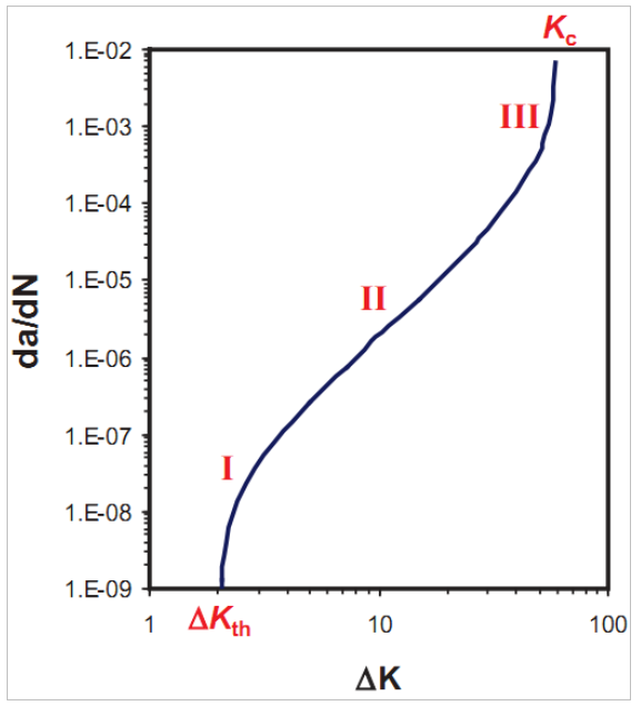
Fig. 5.4.8 Typical fatigue crack growth curve

The crack length \(a(t)\) as a function of time (or number of cycles) can be calculated iteratively based on Eq. (5.4.51). There are three possible failure criteria associated with crack growth:

1. Crack instability: It occurs when \(K_{\max}\left( a(t) \right)\) exceeds the relevant fracture toughness \(K_{instability}\), which depends on the crack geometry, stress/strain state and the environment.

2. Yielding: It occurs if the net section stress \(\sigma_{n}\left( a(t) \right)\) exceeds the flow stress \(\sigma_{flow}\), defined as the average between yield and ultimate stress.

3. Crack size: As an optional criterion the maximum allowable crack size \(a_{\max}\) can be checked.

To perform a reliability analysis, each failure criterion should be evaluated individually. In principle, this evaluation has to be made at every iteration to obtain correct reliability estimates as a function of time. However, in practice it can be sufficient to estimate the probability of failure at discrete time steps, e.g. at the end of each load event or mission phase.

When considering each failure criterion individually, the formulation of limit state functions for a given crack length \(a(t)\) is straight-forward (variable definitions have been given in the definition of the three failure criteria above:

Equation

(5.4.52)\[g_{1}\left( \mathbf{X},a(t) \right) = K_{instability} - K_{\max}\left( a(t) \right)\]

Equation

(5.4.53)\[g_{2}\left( \mathbf{X,}a(t) \right) = \sigma_{flow} - \sigma_{n}\left( a(t) \right)\]

Equation

(5.4.54)\[g_{3}\left( \mathbf{X,}a(t) \right) = a_{\max} - a(t)\]

Different cases should be distinguished to determine the fracture toughness \(K_{instability}\):

• For through cracks: \(K_{instability} = K_{c}\),

• For part-through cracks: \(K_{instability} = K_{Ie}/(a - tip)\) or \(K_{instability} = K_{Ie}/(c - tip)\),

• For part-through crack tips that have free surfaces: \(K_{instability} = 1.1K_{Ie}\),

• For corrosive environments (e.g. Stress Corrosion Cracking): \(K_{instability} = K_{eac}\).

Where, \(K_{c}\) denotes the low constraint toughness value, \(K_{Ie}\) the apparent surface flaw toughness and \(K_{eac}\) corresponds to environmentally assisted crack toughness.

Finally, the probability of failure is estimated by combining all required criteria, e.g. (if only the first two criteria, crack stability and yielding, apply):

Equation

(5.4.55)\[P_{f}(t) = \text{Pr}\left\lbrack g_{1}\left( a(t) \right) \leq 0 \cup g_{2}\left( a(t) \right) \leq 0 \right\rbrack\]

As an alternative, \(g_{1}\) and \(g_{2}\) can also be combined into a single limit state function by making use of an interaction model, as described e.g. by [BR_MEC_26]. Note, however, that these models are generally developed for a specific crack geometry, e.g. assuming a through crack in an infinite plate. Hence, the applicability to the crack under consideration shall be assessed when using an interaction model instead of Eq. (5.4.55).

Independent of the approach chosen to combine several failure criteria, reliability is best assessed using Monte Carlo simulations with variance reduction techniques to reduce the number of required simulations. {term}}FORM/SORM techniques are not recommended due to the iterative nature and nonlinear behaviour of the crack growth model.

To perform a reliability assessment, the following uncertainties should be considered and propagated through the model:

• Loading uncertainty,

• Initial crack size uncertainty,

• Uncertainties associated with material properties.

The probabilistic modelling should explicitly account for the main uncertainties related to each of these three modelling areas.

Uncertainties associated with the loading

For a given crack size and geometry, the stress intensity factor \(K\) is proportional to the stress. Therefore, the uncertainties in the loading can in principle be modelled using the same approach as for the S/N-Curve approach (Section 5.4.7.2.1), i.e. based on a global stress scaling factor \(SSF\) applied to each stress intensity factor during the calculation. However, a more rigorous treatment of the loading sequence is required for crack growth analysis than for the S/N curve approach.

One possible reason for load sequence effects is that the crack growth model predicts larger final crack sizes for a load sequence starting with the largest load amplitudes than for another load sequence with the same load spectrum but starting with the smallest amplitudes. These effects are best considered in a simulation framework, where the whole load process should be simulated for each calculation.

The simulated load sequence can also be used to assess the failure criteria related to crack instability and yielding.

Note

The maximum stress intensity factor \(K_{\max}\left( a(t) \right)\) and the net section stress \(\sigma_{n}\left( a(t) \right)\) in these criteria depends not only on the crack length, but also on the applied maximum stress level \(S_{max}\), leading to a time variant reliability problem.

A simplified, conservative approach to determine the probability of failure during a certain load event or mission phase is to combine the simulated crack length at the end of the considered time interval with the simulated maximum stress level during the same interval when assessing the limit state functions \(g_{1}\) and \(g_{2}\).

Uncertainties associated with the initial crack size

Mechanical parts of space products are usually inspected for defects, using one of the available non-destructive evaluation (NDE) techniques. Nevertheless, even if no defect was detected during the inspection, it cannot be assumed that the inspected part is free of cracks. A probabilistic model for the crack size distribution after inspection can be derived based on the following assumptions:

• A crack is always present, even though it might be very small,

• The crack aspect ratio is known, allowing to focus on a single variable \(a\) to describe the crack,

• The probability distribution of the crack size before inspection is \({f'}_{A}(a)\),

• The uncertainty associated with the chosen NDE technique can be described with the aid of a probability of detection curve \(POD(a)\), see e.g. [BR_MEC_30],

• Only parts without detected defects are used.

Bayes’ theorem (Part 2 - Methods) can now be used to determine the probability distribution of the crack size after inspection [BR_MEC_34]:

Equation

(5.4.56)\[{f''}_{A}(a) = \frac{\left( 1 - POD(a) \right) \cdot {f'}_{A}(a)}{\int_{0}^{\infty}{\left( 1 - POD(a) \right) \cdot {f'}_{A}(a)\text{\ d}a}}\]

In practice, the prior \({f'}_{A}(a)\) will often have to be determined based on expert judgment, as data on the crack size distribution before inspection is generally limited. In the case of a part that is inspected (again) after testing, a probabilistic crack growth analysis for the applied test loads can be used to derive \({f'}_{A}(a)\).

In [BR_MEC_26], [BR_MEC_4] it is stated that the POD curve can be interpreted directly as the cumulative distribution function of the crack size after inspection. This approach leads to the same result as Eq. (5.4.56) when assuming a noninformative (positive) uniform prior distribution for the initial crack size.

Further simplifications are possible if only the NDE limit value is used, which is usually associated with a POD of 90% at a 95% confidence interval. For a given distribution type and coefficient of variation, a probabilistic model for the crack size \(a\) can then be derived by requiring that the exceedance probability of the limit value should be equal to 10%.

Uncertainties associated with material properties

The NASGRO equation parameters \(C,n,p\) and \(q\) are empirical constants whose distribution can in principle be derived from data analysis using experimental data. In practice the problem can be simplified by focusing on those parameters that are relevant for the considered loading and initial crack size, keeping the remaining parameters constant. To give an example, focussing on the Paris law region of the NASGRO equation (region II in Fig. 5.4.8) is acceptable if it is expected that most of the crack growth will occur in this region (i.e. for intermediate initial stress intensity factor ranges and small enough initial crack size). The strongest possible simplification in this case is to model only the multiplicative factor \(C\) as a random variable, summarizing all uncertainties associated with the NASGRO equation.

Apart from the NASGRO equation parameters, also the material properties entering the calculations can be treated as random variables which can be assessed based on experimental data. The sensitivity of these variables on the overall result depends on the loading and the initial crack size.

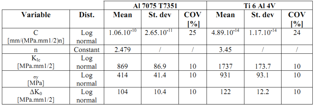
To give an example, the uncertainty associated with the threshold stress intensity factor range \(\mathrm{\Delta}K_{th}\) (e.g. derived from the distribution of \(\mathrm{\Delta}K_{0}\) in Table 5.4.16) can be neglected if the loading does not contain a large number of cycles with stress intensity factor ranges below this threshold.

At the upper limit, uncertainty in the fracture toughness (\(K_{Ic}\) or \(K_{instability}\)) and flow stress \(\sigma_{flow}\) (or yield stress \(\sigma_{y}\)) can be expected to play a major role only if the initial crack size is close to the critical size [BR_MEC_26].

A literature survey presented by Mattrand [BR_MEC_26] reports coefficients of variation between 5% and 25% for the fracture toughness and yield strength of metallic materials

Note

That some material specific information can be found e.g. in MMPDS-12 [BR_MEC_27] or its predecessor, MIL-HDBK-5 [BR_MEC_23].

Typical distributional assumptions for the two variables are Weibull or lognormal distributions. A proposal for the probabilistic modelling of Al 7075 T7351 and Ti 6Al 4V material properties can be found in Table 5.4.16 (taken from [BR_MEC_26]).

Table 5.4.16 Probabilistic modelling of material parameters for Al 7075 T7351 and Ti 6Al 4V

5.4.7.3. Modelling of failures due to corrosion

Compared to terrestrial applications, the relevance of mechanical failures due to corrosion is generally small, as space systems operate in vacuum and a short exposure to corrosive environments on ground is ensured by specific storage conditions. Special types of corrosion that that are of relevance only for specific parts, e.g. in the propulsion subsystem, are not discussed in the present handbook. The reader is referred to the compendium of limit states for space applications that has been prepared by Kowal [BR_MEC_22], which includes also a discussion of several types of corrosion.

A corrosion mechanism that is closely related to the crack growth phenomenon is Stress Corrosion Cracking (SCC), which is defined as an environmentally induced formation and growth of cracks in materials exposed to a corrosive environment. The standard strategy to avoid failures due to this phenomenon is based on the selection of suitable materials, making use of a test-based classification by susceptibility to SCC. Quantitative reliability prediction for this failure mechanism is difficult, even though the effect of the environment can in principle be accounted for in crack growth modelling, see Section 5.4.7.2.2 for details.

5.4.7.4. Modelling of failures due to material degradation

Material degradation is a time-dependent process leading to a reduced performance of materials (deterioration of the physical properties) under the influence of environmental actions such as temperature or radiation. For normal mission durations, these effects can usually be controlled during the design, e.g. by appropriate material selection. However, a dedicated modelling can be required for specific applications, or more broadly for degradation modelling in the context of lifetime extensions beyond the nominal mission.

Thermal degradation is of relevance mainly for non-metallic materials such as polymers or insulation material. Some basic models have been reviewed in [BR_MEC_22]. Thermal degradation as an individual failure mechanism is not discussed any further in the present part.

Note

Temperature can have to be considered as a contributor or influencing variable during several other failure mechanisms, e.g. affecting strength and elasticity parameters for common materials.

The following paragraph provides a brief discussion of radiation degradation and proposes a generic modelling approach for its modelling in mechanical reliability predictions.

5.4.7.4.1. Radiation degradation modelling

The spacecraft radiation environment is characterized by the type, fluence, dose rate, energy spectrum and spatial distribution of nuclear radiation at the considered point of interest inside and outside the spacecraft for the duration of the mission. However, the response can be related directly to the absorbed dose. The dose should be calculated taking both external and internal radiation sources into account.

Radiation affects a variety of material parameters including yield strength and ultimate stress, creep, fatigue, thermal conductivity, hardness, optical properties etc. Metallic materials are rather unaffected by radiation, but degradation needs to be considered for optical materials (e.g. darkening of glass) and for organic materials such as plastics and polymers [BR_MEC_8]. Due to the complexity of the phenomena, a quantitative estimation of the radiation effects is difficult.

Therefore, a simplified assessment of the radiation hardness is performed during the design, taking its basis in an allowable radiation dose, above which the material exhibits significant change in properties. A similar philosophy can be employed for the reliability assessment.

In this case, the difference between the radiation dose \(D\) and allowable dose \(D_{A}\) is used as a limit state function:

Equation

(5.4.57)\[g\left( \text{X} \right) = X_{1} - \Theta \cdot X_{2}(t) = D_{A} - \Theta \cdot D(t)\]

Thus, \(X_{1}\) is defined as the allowable radiation dose \(D_{A}\) and \(X_{2}\) as the cumulated dose \(D\) determined as a function of time \(t\).

Simplified radiation degradation model

A strongly simplified assessment can be achieved by summarizing all uncertainties associated with the radiation modelling in the model uncertainty variable \(\theta\), allowing to consider both \(D\) and \(D_{A}\) in Eq. (5.4.57) as deterministic variables. The resulting simplified model should be seen mainly as a starting point or placeholder for a more detailed modelling.

The variable definitions are given in Table 5.4.17 below.

Table 5.4.17 Assumed probabilistic models for the simplified radiation degradation model

Variable	Definition of the variable	Unit	Distribution	CoV range
\(D_{A}\)	Allowable radiation dose	[rad]	Deterministic	\(-\)
\(D\)	Calculated radiation dose during mission	[rad]	[rad]	\(-\)
\(\Theta\)	Model uncertainty	[\(-\)]	Lognormal	\(\nu_{\Theta} = 0.4\)

To account for the uncertainties in choosing the deterministic values for \(D\) and \(D_{A}\), the coefficient of variation for the model uncertainty is larger than for the other simplified models presented in Section 5.4.7.1 to Section 5.4.7.2. The model uncertainty CoV can be reduced if the model is improved by considering \(D\) and/or \(D_{A}\) as random (instead of deterministic) variables with appropriate uncertainty quantification.

With deterministic dose variables, the expected values of \(X_{1}\) and \(X_{2}\) are simply derived as \(\mu_{X_{1}} = D_{A}\) and \(\ \mu_{X_{2}} = D\); the corresponding coefficients of variation are assumed equal to zero. With these assumptions, the analytic solution for the probability of failure is derived as follows:

Equation

(5.4.58)\[P_{f}(t) = \text{P}\left\lbrack X_{1} - X_{2}(t) \cdot \Theta \leq 0 \right\rbrack = \text{Φ}\left( \frac{\text{ln}\left( \text{E}\lbrack\Theta\rbrack \right) - \text{ln}\left( \frac{\mu_{X_{1}}}{\mu_{X_{2}}} \right) - 0.5 \cdot \text{ln}\left( v_{\Theta}^{2} + 1 \right)}{\sqrt{\text{ln}\left( v_{\Theta}^{2} + 1 \right)}} \right)\]

The main assumptions underlying the simplified radiation degradation model are the following:

• Failure occurs if the cumulated radiation dose exceeds the allowable dose limit.

• All uncertainties associated with the cumulated and allowable dose and their determination are summarized in the lognormal distributed model uncertainty variable.