3.4.3.2. Mission profile#
As mentioned before, the approach followed in this handbook for EEE components is based on the FIDES 2022 guide.
The following paragraphs will mainly address the mission profiles for satellites, probes and crewed vehicles, to account for the specificities of the space environment (see icons on the top left of this paragraph – it applies for its subparagraphs). For launchers, the main phases of the profile being on ground, the recommendations from FIDES 2022 can be followed.
3.4.3.2.1. Mission profile definition#
One advantage of the FIDES approach is that the reliability calculations are specific to a particular application of the electronic equipment or the system, as defined by an application specific mission profile. The consideration of the mission profile allows different reliability prediction results for each unit/subsystem, depending on the actual mission of the spacecraft. In particular, modelling for different mission profiles means taking into account the thermal cycling specific to the orbit considered. The objective of this paragraph is to provide a methodology to define the mission profile of a spacecraft. Some examples of mission profiles for the most common space applications: geostationary (GEO) telecommunication satellites and low Earth orbit (LEO) satellites are presented in Annex A.2.11. The failure rates calculated with FIDES are called calendar Failure Rates, representing the behaviour of the element under consideration over the whole mission profile. Hence, the repartition in time between the different phases impacts the FR obtained. The mission profile can be considered as a whole, to obtain an overall failure rate, related to the whole mission, or the different phases can be considered separately, and it is up to the user to combine the failure rates obtained.
For example, let’s consider a mission composed of three phases A, B, C. If we consider the failure rates FRs of each phase individually we obtain FRa, FRb and FRc, not specific to a time duration. Then, if we considered the whole mission profile, with the % of time spend in each phase x, y, and z, the overall Failure Rate corresponds to (\(x \cdot GF + y \cdot SF + z \cdot GB)/(x+y+z)\). It is up to the user to choose which is the most convenient way to calculate it for their purpose; but it is important not to forget that the time duration of the phases is accounted for in the calculation.
3.4.3.2.2. Methodology to define a mission profile for space applications#
Defining the mission profile, or life profile, is an important step to consider when using FIDES, hence when using the method adapted to space applications, as proposed here. The mission profile allows taking into account the use, which is one of the three items with technology and process on which the reliability prediction of any electronic equipment is based. The mission profile should be as accurate and as pertinent as necessary to get the desired level of confidence in the reliability prediction.
The stress values defined for each phase of the mission profile are used as input parameters describing the physical stresses acting on the EEE components. More specifically, the values of temperature, temperature cycling, vibration and humidity are directly used in the physics of failures equations used in the models for EEE components. The chemical values are used in the consideration of over-stresses with the induced factor \(\Pi_{\text{induced}\_i}\) defined in Section 3.4.3.2.17.
For space applications, such as satellites, probes, crewed vehicles, mission profiles are based on the same main phases, as explained in Section 3.4.3.2.1. Furthermore, the stress applied on electronic equipment of spacecrafts is mainly linked to the temperature, in addition to the electrical stresses dealt with directly at part level. From the regular mission profile definitions from FIDES, the other stresses such as vibrations, humidity and chemical pollution are considered, but they are mainly present only during the launch phase.
So, defining the mission profile of some electronic units used within spacecrafts consists mainly in defining the temperature applied on this electronic equipment (including the thermal amplitudes of the cycles). As these temperatures depend on the equipment, it is not possible to define a standard mission profile that can be used for every piece of equipment within a spacecraft. A minimum of analysis must be done to define the temperatures, leading to reconsider the mission profile for any other equipment or any other mission.
A preliminary simplified mission profile can be defined early in the development process when the required information is not yet fully available.
At that early stage, the definition of this preliminary mission profile can be based on:
A previous mission profile from a similar and preceding mission,
A mission profile for comparison purpose based on examples provided in Annex A : General formulae for EEE components (A.2.11), to use with precautions with regard to the user’s actual use conditions).
WWith the development of the project, thermal simulations are made available by thermal architects and should be used as the basis for the mission profile determination, as much as possible without considering the margins.
So, to define accurately the mission profile, it is necessary to know:
The type of environment of the satellite such as GEO, LEO, medium Earth orbit (MEO), or other kind of trajectories,
The different phases of operating modes and non-operating mode,
The location of the equipment on the platform or on the payload in order to estimate all the relevant stresses.
After that, the mission profile should provide the following data for each phase of life of the electronic equipment in the satellite.
Note
For the non-operating modes, all the Pi-stresses (thermal, mechanical, humidity…) are forced at 0.
|
|||||||||||||||||||||||||||||||||||||||||||||||||||
3.4.3.2.3. Quantification of time data#
The total time \(t_{\text{total}}\) is composed of several phases with duration \(t_{\text{phase}}\).
For most spacecraft applications, the total time \(t_{\text{total}}\) considered for the mission profile of the satellite is the time which normally begins with the launch of the satellite and finishes at the end of its life.
The different phases corresponding to the integration and testing of the spacecraft and its equipment on ground are generally not considered; indeed, the time on ground is generally negligible compared to the mission time and all potential failures arriving during these phases can normally be detected and should not have any impact on the equipment in orbit. But it will be addressed here as in some cases, when the time of storage is significant, it should be considered.
Storage
Hence, the potential storage of spacecrafts before launch can be considered as a specific phase if this one lasts for a long time relatively to the other phases. Some satellites are built and stored waiting for their launch or a satellite is stored during a long duration waiting for an approval to launch. In these specific cases, defining a specific phase of storage is relevant and its duration is defined with the worst case of the duration of storage. For this phase, the electronic equipment is switched off and the temperature and humidity rate are those of the room where the spacecrafts are stored. Normally, there should be only very low controlled variations of temperature, no vibration and no chemical stress.
Decommissioning
The phase of decommissioning should not be considered in regard to the success of the mission, but it could be considered for the success of the disposal process. This occurs at the end of life of the satellite and consists in deorbiting or re-orbiting the spacecraft by changing its orbit to redirect the spacecraft into the atmosphere or in the deep space after passivating all sources of energy.
Only the electronic units used for decommissioning should be taken into account in the reliability prediction for this phase. Also, it is necessary to qualify electronic equipment used for decommissioning in order to be sure that equipment is correctly operating when needed.
Life extension
The potential life extension of a spacecraft is also generally not considered in the initial mission profile. However, it can be considered to forecast reliability during life extension. Therefore, once in orbit, it can be useful to reconsider the reliability prediction to support decisions about lifetime extensions, using a Bayesian approach by considering the past failures of the electronic equipment as described in Part 2 - Methods of this handbook). In this way, the calculation is performed to study the influence on reliability prediction of the additional life. In addition, as described in paragraph 8.6, an analysis should be performed to identify the EEE components with limited life duration, to estimate the potential degradation of the equipment and to mitigate the possible risks of using these components and equipment during the life extension.
Sequence of phases
The sequence of phases is similar whatever the category of satellite except for science missions which can have a different sequence. Phases generally considered in the mission profile are the following for geostationary and low Earth orbit satellites:
Launch phase with duration of around 2 hours: the particularity of this phase is linked to the level of vibration which depends on the launcher,
The next phase is the time to reach orbit, or orbit raising phase: the duration of this phase spans from 2 days up to 1 year according to the technology of propulsion (electrical or chemical). During that phase, units can either be switched on or switched off depending on their purpose,
Once in orbit, the duration of the phases depends on the way the equipment is used with the successive on and off phases and with the category of satellite.
Typically, the orbit duration is between 7 to 12 years for an observation satellite and 10 to 15 years for a geostationary satellite. It can be lower for mini or nanosatellites, and higher for scientific missions.
For each phase, the state of the electronic equipment is specified in the column “On / Off”. If the equipment can be on or off during the same phase, it means that actually two different phases need to be created. The equipment is considered On when its power is supplied, and Off when it is not. The duty cycle corresponds to the ratio of time On over the time Off. For instance, if some unit presents a duty cycle of 60% in-orbit during 5 years (5 times 8760h = 43800h), it is necessary to create two phases, one for the ratio On (60% = 26280h) and one for the ratio Off (40% = 17520h).
Note
Some phases, such as the launch phase, can be removed to simplify the mission profile when these phases have a low contribution on the total prediction.
3.4.3.2.4. Quantification of temperature data#
The thermal characteristics of the electrical equipment in a spacecraft are the main factors of stress, in combination with the electrical stresses at part level. The temperature of the electronic equipment is linked to the environmental temperature outside the satellite and to the regulated temperature inside the satellite.
The environmental temperature of the spacecraft is changing according to the position of the satellite to the sun. The external temperature of the satellite can reach +100°C in the sun light and -200°C in the shadow. That is the reason why a thermal regulation is implemented, in order to have a temperature inside the spacecraft that allows the correct functioning of all equipment. This thermal regulation is generally performed with heating resistance using conduction to heat this equipment. With the ageing of this heating system, it is generally noticed that the temperature of electronic equipment is slightly increasing by several degrees during the life of the satellite.
In the mission profile, the temperature of the electronic equipment is mainly based on this regulated temperature and eventually mitigated by the influence of the environmental temperature, which is used as the reference temperature for the electronic equipment in the proposed models. For each of the electronic boards and for each phase of the mission profile, a reference temperature is defined based on the temperature gradient from the electronic equipment to the electronic boards. If the temperature of the boards inside the equipment is accessible thanks to thermocouples or other sensors, then it is better to directly use this measured temperature in the mission profile. Otherwise, the temperature gradient should be estimated from calculation, thermal analysis and simulation or tests on ground. Finally, the reference temperature of all EEE components is calculated from the reference temperature of each electronic board by considering the temperature rise due to heat dissipation of these components.
When necessary, if the temperature is different depending on the time due to functioning and non-functioning phases, due to ageing of the thermal regulation system, or due to the periods of the year especially close to solstices, then additional phases can be added to reflect the different temperature values.
When the reference temperature is not stable during a phase, for example during activation of an electronic board or an EEE component, the assumption is made that the reference temperature is stable over the whole phase. In this case, the reference temperature to consider is the average temperature during the phase and not the maximum temperature during the phase. During the launch and orbit raising phases, some electronic equipment is switched off and so the temperature is directly the reference temperature of the heating system. As previously noticed, the temperature of the equipment increases with the ageing of the heating system. To consider this phenomenon, an approach in three steps can be followed:
The first step is to define a split into several in-orbit phases with different temperature values from the beginning of life to the end of life of the spacecraft,
The second step is to perform the reliability prediction and to estimate the influence of each phase on the overall reliability prediction,
The third step is to make a simplification in the number of phases by gathering the phases which are less significant.
The domain of applicability for modelling with the proposed method as indicated in the FIDES handbook is -55C to +125C.
3.4.3.2.5. Quantification of temperature cycling data#
The temperature variations at satellite level can be due to:
The successive orbit cycles around the Earth;
The position of the satellite in front of the Sun or in the eclipse of the Earth, depending on the season.
TTo define the different parameters of temperature cycling, it is suggested to define a thermograph for each phase of the mission profile. This thermograph is a direct interpretation of the thermal analysis and simulation done during the preliminary design of the satellite by considering the different phases of the mission profile. The temperature is oscillating around the reference temperature of each electronic board.
A cycle usually corresponds to a temperature excursion measured compared to the reference temperature of the electronic board, and the cycle time is applicable until returning to the initial temperature. This temperature cycle corresponds to an identified phenomenon that generates stress.
Generally, cycles for satellites correspond to a revolution around the Earth. Several identical cycles can succeed in a single phase and the number of identical cycles is counted.
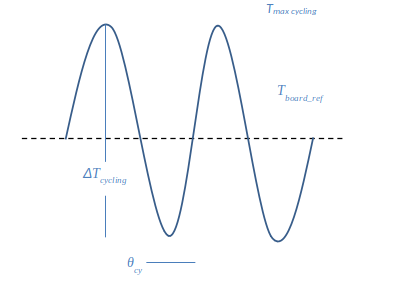
Fig. 3.4.3 Description of temperatures for temperature cycling#
The maximum temperature to be computed for the mission profile corresponds to the highest temperature reached by the electronic equipment during the cycle. The number of cycles is estimated with the total duration of each cycle, and the overall duration of the in-orbit phase.
The domain of applicability for modelling with the proposed method as indicated in the FIDES handbook is:
And,
With a thermal transition rate inferior or equal (\leq) to 20°C.
3.4.3.2.6. Quantification of relative humidity (RH)#
Humidity can only be present during the launch phase and all the phases on ground. Once the spacecraft is in space, there is no more humidity in the environment, and so no more humidity on the electronic equipment. Therefore, it is proposed to consider humidity in the mission profile only during the launch phase and the phases on ground. However, even if the influence of the humidity is light due to the low duration of this phase, the humidity must be considered during this phase. Especially, the relative humidity factor can become predominant in mission profiles of satellites that include long storage periods before launch. That is why the values for relative humidity and temperature shall be determined with accuracy for long storage phases.
In estimating relative humidity, it is important to consider the relative humidity actually experienced by the EEE components. Change in humidity is a function of temperature. For a constant composition of the air, the humidity decreases as the temperature increases. The change in the relative humidity as a function of the temperature can be read from the following hygrothermal diagram.
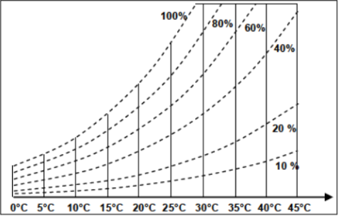
Fig. 3.4.4 Hygrothermal diagram of relative humidity.#
The humidity stress is required for the reliability prediction of sensitive components such as plastic film capacitors, connectors, piezoelectric devices, filters, fuses, integrated circuits, resistors, opto-couplers and PCBs. The theoretical validity range is from 0% to 100%.
3.4.3.2.7. Quantification of vibrations#
The vibrations are mainly present during the launch phase. Once the spacecraft is in space, there is only little vibration and failures due to vibrations are considered as random failures. So, vibrations are mainly considered in the mission profile during the launch phase and can be considered as extrinsic failures. The value of vibrations depends on the position of the electronic equipment inside the satellite, on the maximum vibrations endured by the spacecraft during the launch, and on the launcher. This value is estimated by measurements or mechanical simulations. Even if the influence of vibrations can be small due to the low duration of this phase, the vibrations must be considered.
Whatever the estimated reliability prediction due to vibrations, as the risk of extrinsic failures due to vibrations is still present, specific qualifications of the equipment should be done to ensure that vibrations cannot affect the behaviour of the electronic equipment. The theoretical value must be below or equal to 40 GRMS.
3.4.3.2.8. Quantification of chemical stresses#
The chemical stresses considered in the definition of the mission profile are the following ones:
Saline pollution: This pollution is mainly present near the seaside or for naval equipment; for space applications, this pollution is relevant during the launch phase only if the launch platform is located near the seaside.
Environmental pollution: This pollution could be considered for equipment located in areas where chemical pollutants are present such as industrial areas, chemical industries, oil and gas industries; for space applications, this pollution is relevant during the launch phase only if the launch platform is close to an industrial area.
Application pollution: this pollution is present in areas where the pollution due to other equipment is present, for example an engine of a vehicle; for space applications, this pollution is not relevant except for some equipment close to thrusters.
Protection level: The protection is linked to the ability of humidity to infiltrate in the EEE components; as humidity is not present in space, the protection level is considered as “hermetic”.
So, pollution could be considered as “low” and protection level as “hermetic” for any electronic equipment in spacecrafts, except for some specific cases, such as the launch phase when humidity and chemical pollution are present. The chemical stresses are required for the reliability prediction of some electromechanical components such as fuses and connectors.
3.4.3.2.9. Exposure to over-stresses#
The contributions of over-stresses in the mission profile on components are defined in Section 3.4.3.2.17 the induced factor \(\Pi_{\text{induced}\_i}\) and application factor \(\Pi_{\text{application}}\).
3.4.3.2.10. Specific stresses not considered in the mission profile#
Some of the stresses should not be considered to the real level of influence that they can have in space applications compared to other applications. The failures due to On / Off cycles and due to radiations are classified as degradation failures, as they affect the degradation of the equipment.
3.4.3.2.11. On / Off cycles#
The equipment is generally switched off when it is not used to limit as much as possible the consumption of energy. In the mission profile, the impact on EEE components of the frequent On / Off cycles are considered only by the thermal variations due to the self-heating of electronic equipment in the model. The influence of frequent switching on and switching off on the reliability of electronic equipment is not perfectly apprehended and not correctly considered. A transmitter of a LEO satellite being switched off when out of the scope of the reception stations can occur up to 100 000 times over the mission lifetime without having any failures. For this specific constraint, no potential impacts have been currently found with experience of IOR. Consequently, the impact of these frequent On / Off cycles is considered as a degradation phenomenon of EEE components and is discussed in Section 3.4.5.5.
3.4.3.2.12. Radiations#
Another specificity of the space domain is an environment subjected to high cumulated doses of radiation (protons and electrons), due to the Van Allen radiation belt in particular. The methodology considers a part of these phenomena through the electrical over-stresses, but with insufficient quantification. Currently, the design of any electronic equipment for satellites is qualified with the total dose corresponding to the life of the equipment with a supplementary safety margin. However, commercial EEE components are more and more sensitive to cumulated doses of radiation.
The experience and lessons-learnt issued from various industrial domains is not sufficient to presently develop these models. For space applications, only simple models such as the model presented in Section 3.4.5.5.1 is proposed with results of radiation tests performed on components correlated with the level of radiation considered in the different phases of the mission profile.
Note
Concerning radiations as well, Single Events Effects (SEEs) are not considered here as they do not result from failures but from deterministic phenomena.
3.4.3.2.13. Temperature and thermo-electrical stress#
Physical stresses
In the classification of Part 2 - Methods of this handbook, the physical failure rate \(\lambda_{\text{Physical}}\) is based on a combined approach. It gathers the following information:
The basic failure rates \(\lambda_{0}\) based on statistics,
The physical contributions \(\Pi_{\text{acceleration}}\) which are based on the physics of failures, as described in Section 3.4.3.2.13, Section 3.4.3.2.14, Section 3.4.3.2.15, Section 3.4.3.2.16,
The contributions of specific over-stresses \(\Pi_{\text{induced}}\) not considered by the mission profile, as described in Section 3.4.3.2.20.
The physical contributors considered are the temperatures, the humidity level, the thermal cycling, the vibrations and the electrical stresses. The formulas applied in the models have been established from the physics of failures of each EEE component considered. The thermal and thermo-electrical stresses are taken into account by the physics of failures with the Arrhenius‘ law, multiplied by the contribution of electrical stress, such as voltage or current for example (see Annex A.2.3 for the acceleration factor equations).
For some components that are sensitive to failure mechanisms linked to electrical operation, the contribution of electrical stress is considered as a multiplicative factor. This electrical stress is determined based on the ratio between applied stress and rated stress, elevated to an accelerating power \(p\). The considered stresses are voltage and current. The accelerating power \(p\) is derived based on publications or by engineering judgment.
3.4.3.2.14. Thermo-mechanical stress#
The thermo-mechanical stress is associated with the thermal cycling of the equipment. It is considered by the physics of failures with the Norris-Landzberg’s model defined in document [BR_EEE_22]. This model is based on the thermo-mechanical effects based on the Coffin-Manson model.
3.4.3.2.15. Humidity stress#
The humidity stress is taken into account by the physics of failures with Peck‘s model
It is presented in Annex A.2-5 and in Formulae concerning section 8.3.5.1 Capacitors, Annex B.1, Equation B.1-10. Peck’s model uses the activation energy \(E_{a}\) and the humidity factor \(p\) as inputs to the calculation of humidity contribution to the reliability prediction. All other parameters are depending on the mission profile of the equipment.
For space applications, the humidity stress is present only during the launch phase (and storage/on-ground phases if they are taken into account). In orbit, humidity is no more present and the stress is no more applied.
3.4.3.2.16. Vibration stress#
The vibration stress is taken into account by the physics of failures with Basquin’s law.
It is presented in Annex A.2-6. This accelerating model uses the power factor p as inputs to the calculation of the vibration contribution to the reliability prediction. The other parameter is depending on the equipment’s mission profile. The vibration power \(p\) is similar for all components and set to \(p=1.5\). This value is close to the bottom of the range of fatigue coefficients generally encountered for Basquin’s law. For space applications, the vibration stress is present only during the launch phase. In orbit, vibrations are no more present and the stress is no more applied.
Recommendation
When computing the vibration input in the mission profile in a tool, for phases with no vibration, it is recommended nevertheless to compute as a minimum 0.01 Grms value for stability of the formulae within the tool.
3.4.3.2.17. Recommended values for over-stresses of EEE components for space applications#
The method recommended here directly considers the contribution of mechanical, electrical or thermal over-stresses on components as described in Section 3.4.3.2.13. An additional factor, the induced factor \(\Pi_{\text{induced}\_i}\) is a parameter representing the contribution of other specific over-stresses not considered by the mission profile. This induced factor is based on four different contributors according to the equation presented in Annex A, section A.2-7.
3.4.3.2.18. Influence of the component placement in the equipment#
\(\Pi_{placement\_ i}\) translates the influence of the component position in the equipment or the system. As described in the FIDES 2022 handbook, in order to determine which Pi Placement applies to a component, two questions need to be answered:
Is the component considered at the interface or not at the interface?
Is the component part of a digital, analog or power function?
To be able to answer the first question, it is important to insist on a common definition of “interface”: An interface is the junction that provides interconnection between two systems. The concept of interface must be considered from an electrical point of view. A component is considered as an interface if it is more exposed to accidental electrical hazards because of its position in the system. On a circuit board, the interface components are often (but not only) protections, filters or insulation components. Should be considered as an interface component all components on an input signal up to the first protection or the first active part able to withstand a surge. For space applications, interfaces are generally functionalities linked to the power bus and data bus shared between platform and payload. Concerning the second question, it is important to insist on the fact that the focus concerns the function that the component is included in, not the component itself. All components constituting the same functional block should inherit the same \(\Pi_{placement\_ i}\). This parameter is defined in Annex A, section A.2-8.
3.4.3.2.19. Influence of the use environment#
\(\Pi_{application\_ i}\) represents the influence of the use environment for the application of the product containing the component. For example, the exposure to a mechanical overstress is more significant in electronics integrated into a mobile system than in a fixed station system. This factor is usually variable depending on each phase of the mission profile. This parameter is based on a list of criteria which have three different levels corresponding to a favourable, moderate or unfavourable situation. For space applications, these criteria can be fixed as the use environment is normally the same for all satellites. In some specific situations, it could be possible to make some adaptations, but normally these values are appropriate whatever the equipment and whatever the phase of the mission profile.
Therefore, the recommendation for space applications during the launch, time to reach orbit and in-orbit phases is the following:
Each level 0, 1 or 2 of the recommendation is given a specific mark as defined in the table, independently of the levels and independently of the phases, as presented in Annex A, section A.2-9.1.
Level |
\(\Pi_{marks\_ k}\) |
|---|---|
0: favourable or non-aggressive |
1 |
1: moderate |
3.2 |
2: unfavourable or severe |
10 |
The final calculation of \(\Pi_{application\_ i}\) is therefore:
Equation
So, the recommendation for space applications for the launch, time to reach orbit and in-orbit phases is to use the value of 1.13 for the calculation of \(\Pi_{application\_ i}\) in all applications.
For transport and storage phases of the mission profile, the Recommendation for space applications is presented in Annex A.2-9.2.
Based on the marks given in Table 3.4.3 and calculation with (3.4.1), the recommendation for space applications for transport and storage phases is to use the value of 1.00 for the calculation of \(\Pi_{application\_ i}\) in all applications.
3.4.3.2.20. Influence of the policy for over-stresses#
\(\Pi_{ruggedising}\) represents the influence of the policy for considering over-stresses in the product development and is based on 17 different questions presented in the paragraph dedicated to \(\Pi_{ruggedising}\) in [NR_EEE_2], page 102.
Some of the answers to these questions are common to all space applications. Questions n° 157, 158, 159, 160, 161, 163, 167 and 169 have been partly modified to consider specificities of space applications, mainly because maintenance of the products is not possible on spacecrafts. The modification of the Recommendations, descriptions and criteria of these modified questions are listed in Annex A : General formulae for EEE components, section A.2-10. Moreover, question n°168 is not directly applicable to space applications also due to its maintenance purpose and is removed from the questionnaire.
Recommendation
Answer all the questions as N4 (“Recommendation is fully applied”) for most electronic units’ suppliers in the space industry, as a first approach.
Rule
For CDR, sub-contractors, or suppliers, in particular those who are new in the space industry or in the frame of “new space” programs need to adapt these levels to their conditions with rationale provided. Therefore, the table with associated weights and levels N4 for space applications is presented in Annex A.2-10, Table A.10-1.
3.4.3.2.21. Coefficient of sensitivity to over-stresses#
\(C_{sensitivity}\) represents the coefficient of sensitivity to over stresses inherent to the item technology considered. Sensitivities related to electrical overstress, thermal overstress and mechanical over stress are given, to show the relative sensitivity of EEE components to the different types of over stresses. The coefficient \(C_{sensitivity}\) is an exponential factor in the \(\Pi_{induced\_ i}\) formula and specific to each component technology. The values for each technology are provided in Section 3.4.3.5.