5.4.8. Examples

The following paragraphs provide some examples for the application of the methods introduced in Section 5.4.6 and Section 5.4.7.

5.4.8.1. Simplified wear modelling: solid lubricant wear

In this example, the simplified method presented in Section 5.4.7.1 is utilized to model the reliability of a bearing. The considered failure mechanism is solid lubricant wear.

Given

A solid lubricated ball bearing is considered. The basic variables, necessary to model the failure mechanism, are modelled as follows:

Table 5.4.18 Variables considered in the example

List of variables Unit Distribution Expected value CoV \(V_{\text{limit}}\) Limiting value (worn volume) \(m^3\) Lognormal \(6\cdot 10^{-8}\) \(0.2\) \(n_P\) Number of phases / time intervals - Deterministic \(1\) - \(K_{H,i}\) Specific wear rate in interval \(i\) \(Pa^{-1}=N/m^2\) Lognormal \(0.6\) \(\alpha_i\) Ball-cage interaction in interval \(i\) \(Nm\) Lognormal \(0.033\) \(0.1\) \(\text{rev}_i\) Number of revolutions in interval \(i\) - Deterministic \(10^{6}\) - \(\theta\) Model uncertainty - Lognormal \(1.2\) \(0.2\)

Note

The values indicated in the following table serve as an illustrative example.

In this example, it is assumed that only one mission phase is relevant, i.e. \(n_P=1\).

Reliability model

To estimate the probability of failure with the simplified methods, the following need to be known:

• The expected value of the limiting volume,

• The CoV of the limiting volume,

• The expected value of the volume worn away

• The CoV of the volume worn away.

According to Eq. (5.4.20), the expected value of the limiting volume is:

Equation

(5.4.59)\[\text{E}\left[ X_1 \right] = \text{E}\left[ V_{\text{limit}}\right ] = 6\cdot 10^{-8}\]

According to Eq. (5.4.22), the coefficient of variation of the limiting value is:

Equation

(5.4.60)\[v_{X_1}=v_{V_{\text{limit}}}=\frac{\sqrt{\text{Var}\left[V_{\text{limit}}\right]}}{\text{E}\left[V_{\text{limit}}\right]}=\frac{\text{E}\left[V_{\text{limit}}\right]\cdot0.2}{\text{E}\left[V_{\text{limit}}\right]}=0.2\]

To calculate the CoV of the volume worn away, the covariance of \(K_H\) and \(\alpha\) is calculated under the assumption of full correlation between \(K_H\) and \(\alpha\):

Equation

(5.4.61)\[\begin{split}\text{Cov}\left[K_H,\alpha\right]&= \sigma_{K_H}\cdot\sigma_\alpha=v_{K_H}\cdot \text{E}\left[K_H\right]\cdot v_\alpha\cdot \text{E}\left[\alpha\right]\\ &=0.6\cdot 4\cdot 10^{-15}\cdot 0.1\cdot 0.033=7.92 \cdot 10^{-18}\end{split}\]

The variance of the product \(K_H\cdot\alpha\) is calculated as:

Equation

(5.4.62)\[\begin{split}\text{Var}\left[K_H\cdot\alpha\right]&=Var_{K_H}\cdot \text{Var}_\alpha+Var_{K_H}E\left[\alpha\right]^2+Var_\alpha E\left[K_H\right]^2\\ &=5.76\cdot10^{-30}\cdot1.1\cdot10^{-5}+5.76\cdot10^{-30}\cdot\left(0.033\right)^2+1.1\cdot10^{-5}\cdot\left(4\cdot10^{-15}\right)^2\\ &=6.51\cdot10^{-33}\end{split}\]

According to Eq. (5.4.22), the expected value of the volume worn away is:

Equation

(5.4.63)\[\begin{split}\text{E}\left[X_2\right]&=\text{E}\left[K_H\cdot\alpha\right]\cdot \text{rev}=\left(\text{E}\left[K_H\right]\cdot \text{E}\left[\alpha\right]+\text{Cov}\left[K_H,\alpha\right]\right)\cdot \text{rev}\\ &=\left(4\cdot10^{-15}\cdot0.033+7.92\cdot10^{-18}\right)10^6\\ &=7\cdot10^{-8}\end{split}\]

And the CoV of the volume worn away is according to Eq. (5.4.23):

Equation

(5.4.64)\[v_{X_2}=\frac{1}{\text{E}\left[X_2\right]}\cdot \text{rev}\cdot\sqrt{Var\left[K_H\cdot\alpha\right]}=\frac{1}{1.4\cdot10^{-10}}\cdot10^6\cdot\sqrt{6.51\cdot10^{-33}}=0.577\]

Finally, the probability of failure is calculated according to Eq. (5.4.24):

Equation

(5.4.65)\[\begin{split}P_f&=P\left[X_1-X_2\cdot\Theta\le0\right]\\ &=\Phi\left(\frac{ln\left(E\left[\Theta\right]\right)-ln\left(E\left[X_1\right]/E\left[X_2\right]\right)+0.5\cdot\left(ln\left(v_{X_1}^2+1\right)-ln\left(v_{X_2}^2+1\right)-ln\left(v_\Theta^2+1\right)\right)}{\sqrt{ln\left(v_{X_1}^2+1\right)+ln\left(v_{X_2}^2+1\right)+ln\left(v_\Theta^2+1\right)}}\right)\\ &=\Phi\left(\frac{ln\left(1.2\right)-ln\left(6\cdot10^{-8}/1.4\cdot10^{-10}\right)+0.5\cdot\left(ln\left(0.2^2+1\right)-ln\left(0.577^2+1\right)-ln\left(0.2^2+1\right)\right)}{\sqrt{ln\left(0.2^2+1\right)+ln\left(0.577^2+1\right)+ln\left(0.2^2+1\right)}}\right)\\ &=\Phi\left(-2.709\right)=0.0034,\end{split}\]

Where, \(\Phi\) denotes the cumulative standard normal distribution.

5.4.8.2. Updating of reliability estimates derived from structural reliability methods

This example is based on the example provided in Section 5.4.8.1, i.e. it considers a bearing that fails from solid lubricant wear. The structural reliability model is established with the simplified methods in Section 5.4.7.1. Upon availability of new data on the reliability of the bearing in question, the model is updated making use of the approach described in Section 5.4.6.5.

Given

A solid lubricated ball bearing is considered. The basic variables, necessary to establish a reliability model in accordance with the simplified method described in Section 5.4.6.2, are modelled as follows:

From Section 5.4.7.1, it follows:

Equation

(5.4.66)\[\text{E}\left[ X_1 \right] = \text{E}\left[ V_{\text{limit}}\right ],\]

And, under the assumption of a single mission phase:

Equation

(5.4.67)\[\text{E}\left[ X_2 \right] = \text{E}\left[ K_H\cdot\alpha \right]\cdot\text{rev} = (\text{E}\left[ K_H\right]\cdot\text{E}\left[ \alpha\right] + \text{Cov}\left[ K_H, \alpha\right])\cdot\text{rev}.\]

Prior model

The probability of failure in function of the number of revolutions \(\text{rev}\) is modelled. According to Section 5.4.6.5, it can be approximated with the lognormal distribution:

Equation

(5.4.68)\[\text{rev}\sim\text{Lognormal}(\mu_{\text{rev}, \sigma_{\text{rev}}}).\]

The CoV \(v_{X_1}\) and \(v_{X_2}\) have already been determined in the example in Section 5.4.8.1.

Equation

(5.4.69)\[\sigma_{\text{rev}}=\sqrt{ln\left(v_{X_1}^2+1\right)+ln\left(v_{X_2}^2+1\right)}=\sqrt{ln\left(0.2^2+1\right)+ln\left(0.577^2+1\right)}=0.571.\]

The location parameter \(\mu_{\text{rev}}\) is considered uncertain and is modelled with a normal distribution (conjugate prior, see Part 2 - Methods).

Equation

(5.4.70)\[\mu_{\text{rev}}\sim\text{Normal}(\mu',\sigma')\]

According to Section 5.4.6.5, \(p=\frac{E\left[X_1\right]}{E\left[X_2\right]}\) should be brought to the form \(p=k\cdot\frac{1}{rev}\). Using the relations in Eq. (5.4.24) and Eq. (5.4.28):

Equation

(5.4.71)\[p=\frac{E\left[X_1\right]}{E\left[X_2\right]}=\frac{E\left[V_{\text{limit}}\right]}{E\left[K_H\cdot\alpha\right]\cdot \text{rev}},\]

(5.4.72)\[k=\frac{E\left[V_{\text{limit}}\right]}{E\left[K_H\cdot\alpha\right]}=\frac{6\cdot10^{-8}}{1.40\cdot10^{-16}}=4.29\cdot10^8.\]

The prior hyperparameters for the distribution of \(\mu_{\text{rev}}\) are estimated according to Eq. (5.4.13) and Eq. (5.4.14):

Equation

(5.4.73)\[\begin{split}\mu\prime&=ln\left(k\right)-ln\left(E\left[\Theta\right]\right)+0.5\cdot\left(ln\left(v_\Theta^2+1\right)-ln\left(v_{X_1}^2+1\right)+ln\left(v_{X_2}^2+1\right)\right)\\ &=ln\left(4.29\cdot10^8\right)-ln\left(1.2\right)+0.5\cdot\left(ln\left(0.2^2+1\right)-ln\left(0.2^2+1\right)+ln\left(0.577^2+1\right)\right)\\ &=19.84\end{split}\]

(5.4.74)\[\sigma\prime=\sqrt{ln\left(v_\Theta^2+1\right)}=\sqrt{ln\left(0.2^2+1\right)}=0.198\]

Additional data

Additional data on the reliability of the bearing is given in the table below:

Table 5.4.19 Additional data considered in the example

Specimen	Revolutions to failure \(\widehat{{\text{rev}}_i}\)
1	\(2.5\cdot{10}^8\)
2	\(2.4\cdot{10}^8\)
3	\(2.7\cdot{10}^8\)
4	\(3.1\cdot{10}^8\)
5	\(3.4\cdot{10}^8\)
6	\(3.8\cdot{10}^8\)
7	\(5.1\cdot{10}^8\)

Updating

With the additional data, the reliability model for the bearing can be updated. The updating is done using the equations for the analytic approach using conjugate priors, given in Part 2 - Methods of this handbook:

Equation

(5.4.75)\[\sigma\prime\prime=\frac{1}{\sqrt{\frac{1}{\left(\sigma\prime\right)^2}+\frac{n_{data}}{\left(\sigma_{rev}\right)^2}}}=\frac{1}{\sqrt{\frac{1}{\left(0.198\right)^2}+\frac{7}{\left(0.571\right)^2}}}=0.145,\]

(5.4.76)\[\mu\prime\prime=\left(\sigma\prime\prime\right)^2\cdot\left(\frac{\mu\prime}{\sigma\prime^2}+\frac{\sum_{i=1}^{n_{data}}ln\left({\widehat{rev}}_i\right)}{\sigma_{rev}^2}\right)=0.146\left(\frac{19.84}{\left(0198\right)^2}+\frac{137}{\left(0.571\right)^2}\right)=19.72.\]

The posterior predictive of \(\text{rev}\) is also a lognormal distribution. Its distribution function can be calculated with the help of the analytic formulas provided in Part 2 - Methods of this handbook.

Results

In Fig. 5.4.9, the prior and posterior distribution of parameter \(\mu_{\text{rev}}\) is represented. In Fig. 5.4.10, the prior and posterior probability of failure are shown in function of the number of revolutions \(\text{rev}\). As can be seen in the figure, the probability of failure increases from the updating.

Fig. 5.4.9 Prior and posterior distribution for parameter \(\mu_{\text{rev}}\)

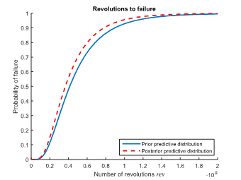
Fig. 5.4.10 Prior and posterior predictive distribution of revolutions to failure \(\text{rev}\)

5.4.8.3. Updating of structural reliability methods using right censored data

In contrast to the example in Section 5.4.8.2, censored data is often available in practice. In this case, the simplified analytic approach for updating is no longer applicable and numerical methods should be used. In this example, MCMC will be used to do the updating for the location parameter. To keep the example simple, the same assumption as in Section 5.4.8.2 is made that the scale parameter is known and will not be updated. This assumption is not necessary using MCMC for the updating and might be relaxed for a more advanced modelling.

Additional data

Additional, censored, data on the reliability of the bearing is given in the table below

Table 5.4.20 Additional censored data for the reliability of a bearing

Specimen	Revolutions to failure \(\widehat{{\text{rev}}_i}\)
1	\(2.5\cdot{10}^8\)
2	\(2.4\cdot{10}^8\)
3	\(2.7\cdot{10}^8\)
4-20	\(\ge 5.1\cdot{10}^8\)

Updating

With the additional data, the reliability model for the bearing can be updated. The updating is done using the MCMC method described in Part 2 - Methods. The data set is right-censored and the likelihood \(L\) for a right censored data set is given by:

Equation

\[L\propto\ \prod_{i=1}^{n}{f\left(\widehat{x_i}|\theta\right)\cdot\prod_{j=1}^{m}\left(1-F\left(\widehat{x_{\text{up}}}|\theta\right)\right)},\]

Using the data from above (Table 5.4.20), the likelihood is given by:

Equation

\[L\propto f\left(2.5\ {10}^8|\theta\right)\cdot f\left(2.4\ {10}^8|\theta\right)\cdot\ f\left(2.7\ {10}^8|\theta\right)\cdot\left(1-F\left(3.4\ {10}^8|\theta\right)\right).\]

Using the additional data, the reliability model for the bearing can be updated. The result of the updating is:

Equation

\[\begin{split}\sigma\prime\prime&=0.1292,\\ \mu\prime\prime&=20.23\end{split}\]

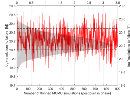
Fig. 5.4.11 Markov chain and posterior density of the parameter

The posterior predictive of \(\text{rev}\) is shown in Fig. 5.4.12. It is seen that the consideration of censored data might have a large impact on the updating and has a large potential especial for end of life decision-making.

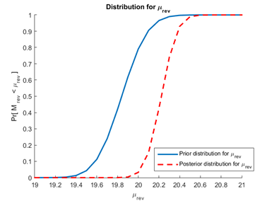
Fig. 5.4.12 Prior and posterior distribution for parameter \(\mu_{\text{rev}}\)

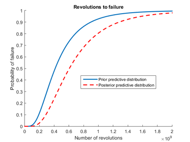
Fig. 5.4.13 Prior and posterior predictive distribution of revolutions to failure \(\text{rev}\)