9.4.9. Systematic failure modelling#
The present paragraph introduces the modelling of systematic failures using IOR data. After an introduction to the topic (Section 9.4.9.1) and the classification of systematic failures (Section 9.4.9.2), the modelling is explained starting with the data sources and methods used (Section 9.4.9.3). The description of the model in Section 9.4.9.4 starts with a discussion of is range of applicability, which is related to the applicability of the data source used.
9.4.9.1. Systematic failures in reliability prediction#
According to the classification provided in Part 2 - Methods, systematic failures are failures for which the root cause is known and has been identified as a design, manufacturing or operations error. The fact that the root cause is known (at least a posteriori) and can be eliminated is the main difference between systematic and random failures. First priority should thus clearly be to avoid systematic failures rather than modelling their occurrence. However, it is also clear that even though a specific root cause can be eliminated by adapting the design or the process in which the error occurred, experience shows that other root causes will lead to new systematic failures. It is thus possible and can be meaningful, depending on the intended use of the prediction, to derive a statistical model for systematic failures in the same way as for random failures.
Another major difference to random failures is that systematic failure root causes can be introduced at any level of assembly, from part to system. In fact, considering the high quality of parts used in space and the complexity and uniqueness of the assembled systems, one can even assume that the occurrence of part related systematic failures is negligible compared to non-part related failures with root causes introduced at higher levels of assembly.
It is important to remind that the occurrence of systematic failures at lower levels of assembly can be driven by common cause effects and it is generally not valid to assume independence between systematic failures, e.g. in identical equipment operating in redundancy. However, two systematic failures resulting from the same root cause should not be fully dependent either; depending on the setting the degree of dependence between two systematic failures can range from nearly independent to fully dependent.
The modelling approach followed in the present paragraph avoids these difficulties by working top-down, starting at spacecraft level and going down to subsystem level only. No common cause modelling is required with this approach, as subsystems are combined at spacecraft level in a serial system design. However, common cause should be considered for systematic failures when relying on models developed at lower levels.
Considering the system level effects, it can be said that systematic failure root causes are generally more likely to lead to severe consequences at spacecraft level than random failures, whose effect can be modelled and mitigated by redundancy and Fault Detection Isolation and Recovery (FDIR). However, this does not mean that each systematic failure immediately leads to the collapse of the overall system in the sense of a single point failure. Redundancy, robust design and failure detection and recovery can help in the case of systematic failures as well, and workarounds can be implemented from ground by uploading software updates and/or adapting operational procedures.
To account for these mitigation measures, the modelling presented in this paragraph considers (major) anomalies rather than failures and works with a classification by severity to model the impact on the mission. Definitions are provided in Section 9.4.9.3.1. Fig. 9.4.33 illustrates the introduction of flaws during design (including specification) and manufacturing, which if undetected before launch, can lead to failures or anomalies in orbit under operational and/or environmental stresses.
Note
Operation errors can lead to systematic failures even without the presence of flaws.
The severity category depends on the effect propagation in the overall system and can be reduced by mitigation measures implemented a priori during design, or a posteriori after anomaly investigation.
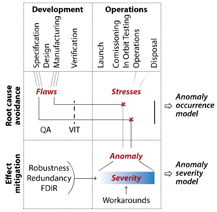
Fig. 9.4.33 Root causes and effects of systematic failures#
An ideal model for systematic failure or anomaly modelling considers all the aspects shown in Fig. 9.4.33, including not only the root causes of failure, but also the effect of mitigation measures implemented to avoid the occurrence of systematic failures and to mitigate their effect on the mission. In the present paragraph, a first step is made, focussing on the occurrence and severity of anomalies in orbit. The resulting model provides global quantitative figures that are already useful for reliability prediction in a top-down approach, but it is does not allow to quantify the effect of the various mitigation measures that have already been implemented before launch.
9.4.9.2. Systematic failures classification#
To define and classify systematic failures, it is first necessary to define a sound “design”, a sound “manufacturing” and a sound “operation”. The related errors are derived accordingly.
“Design” is sound when the system:
Performs the functions and the performances specified in the technical specification,
• Is able to sustain / handle all the stresses: internal (by design, according to the elements user manuals) and external (“normal” environment) as specified (= “under given conditions”) during the design lifetime, when operated without any misuse (in consistency with the user’s manual).
E.g. design error = weakness in design creating electrical overstresses on electronic parts up to definitive failure of the part.
“Manufacturing” is sound when the “as-built” system:
• Respects the design characteristics, i.e. key characteristics (design assumed sound), i.e. no defect. E.g. Manufacturing error = defect in a soldering leading to increased impedance inducing increase of voltage drop and reduction of current.
“Operation” is sound when the “as-built” system:
• Is used / operated in conformance with the user’s manual (assumed to be sound, user’s manual is considered as part of design): o Mission profile consistency, o As per design definition, neither overstresses nor additional/external stresses.
E.g. operation error = 300 000 On/Off cycles over mission lifetime whereas the part is qualified with respect to 100000 On/Off only.
Note
The term “system” in this context can relate to different levels in the system hierarchy, e.g. equipment, subsystem or spacecraft level.
Systematic failures can result from requirement, design or manufacturing errors not identified during verification, or from operations errors after launch. Also software errors fall into this category. The common characteristic is the failure root cause, which is human error, or possibly a tool issue either tool-supported prediction, modelling for design or tool-supported integration for manufacturing errors. The main difference between the different categories is the process during which the error is introduced:
• Design errors during design phase (including requirement specification),
• Manufacturing errors during manufacturing phase,
• Operations errors during operational phase.
Note
The same categorization in principle applies also to software errors, which can be introduced during software requirement specification, during software design and during manufacturing (coding). During operations (maintenance), software errors can be introduced when uploading patches, including errors that occur during the process of uploading the patch.
Independent of the classification, all types of errors can lead to failures in-orbit, i.e. during operations, if they are not identified and successfully eliminated, during the verification phase (design, manufacturing error).
In principle, systematic failures can be introduced at any level. This holds especially for design and manufacturing errors, which can result from weaknesses in the design or manufacturing of parts, equipment, interfaces or the overall system. At spacecraft level, operation mistakes and software errors come into play. It should be noted that the level at which a failure is observed can be different due to failure propagation processes.
Note
In some situations, the systematic failures occur in a complex failure scenario, e.g. a random failure at equipment level can lead to the loss of the satellite through failure propagation when the FDIR function is not designed appropriately (e.g. no segregation between nominal channel and redundant one).
9.4.9.3. Data sources and methods#
It is important and not necessarily easy to select wisely the data sources and methods to model this type of failures.
9.4.9.3.1. Inputs used for modelling#
The data source used for quantitative modelling of systematic failures is in-orbit return (IOR) data with information on major anomalies collected at satellite level. A fundamental assumption for the use of IOR is that the occurrence of systematic anomalies in orbit depends on the quality assurance policy and processes implemented in the space industry, allowing to use information from the past as long as the processes do not change fundamentally.
Relying on the inputs from a given data source, the modelling results obviously depend on the classification of anomalies and failures used to generate the data sample. In particular, the classification of an event as “systematic” or “random” plays an important role in this context, and can be based on very different criteria in different organizations, even when working with the same definitions.
All classifications and definitions required to understand the modelling are provided in the following.
Example of major anomaly
The term “anomaly” is defined as any deviation from the expected situation. It includes failures, but also other events like e.g. outages or erroneous functioning.
The following anomalies observed in orbit are classified as major:
• A hardware definitive failure at equipment level, total or partial
• A FDIR inadvertent triggering leading to hardware configuration modification
• An outage (mission is stopped during a certain time, or the operation plan is not respected)
• A definitive loss of more than 20% of the mission
Classification of anomalies as “systematic”
The models and data presented in this paragraph are consistent with the classification of failures by root cause discussed in Part 1 - Methodologies of this handbook; the classification of anomalies is based on the same principles. Only major anomalies classified as “systematic” are considered for the modelling. As discussed in Section 9.4.9.2 above, this includes anomalies due to errors in the design (including specification), manufacturing and operation of space systems.
Classification of major anomalies by severity (satellite level)
The data used for modelling provides information on anomalies observed during operations in orbit. Combined with data on the fleet (providing information on the satellites’ lifetime), this anomaly data is used to derive the anomaly occurrence rate as a function of operating time. It is important to note that also anomalies without mission impact are considered in the occurrence model, with the aim to achieve a more relevant sample size. The following five severity classes are used to classify the anomalies by their effect on the mission:
Severity 1, High: Impact on mission between ]50% - 100%]\
A « mission high critical » event leads, at the end of the failure scenario, to the loss of more than 50% of the mission (versus major performances) as defined in the Technical Specification.
Severity 2, Medium: Impact on mission between ]10% - 50%]\
A « mission medium critical » event leads, at the end of the failure scenario, to the loss of more than 10% and less than 50% of the mission (versus major performances) as defined in the Technical Specification
Severity 3, Low: Impact on mission between ]0% - 10%]\
“A « mission low critical » event leads, at the end of the failure scenario, to the loss of more than 0% and less than 10% of the mission (versus major performances) as defined in the Technical Specification.
Severity 4, No impact: No mission impact, with hardware failure (recovery/workaround)\
The anomaly can lead to mission interruption or not, with definitive HW failure and mission fully resumed at the end of the failure scenario (recovery/workaround).
Severity 5, None: No mission impact, without hardware failure\
The anomaly can lead to mission interruption or not, without definitive HW failure and mission fully resumed at the end of the failure scenario.
Note
In the case of Single Point Failure (SPF) (i.e. no redundancy), a definitive failure would lead to severity from 1 to 3, depending on the consequences.
For severity level 1 (high critical) to severity level 3 (Low critical) the percentage of the mission impacted should be defined in the frame of the satellite. To give an example, the loss of 30% of the power is easily ranked to level 2, even though the power budget encompasses BOL margin; a satellite unable to reach its nominal orbit is considered as severity class 1, even though in some cases it could be possible to adapt the mission to these unplanned conditions.
Anomalies with no impact on the mission (Severity 4 and 5) are further classified as involving a definitive hardware failure at lower levels (e.g. loss of redundancy at equipment level) or not. Anomalies classified as Severity 1, 2 or 3 can not involve a definitive hardware failure in the strict sense but could be considered as not respecting the technical specification, and thus as failures in the wide sense. Thus, for modelling purposes it is assumed that in besides anomalies classified as Severity 4 (no impact, with hardware failure), anomalies with mission impact >0% do necessarily involve a hardware failure (in the wide sense) as well.
It should be noted that even though there is no difference in terms of the consequences at system level between the severity categories 4 and 5, from a reliability perspective (considering the remaining lifetime after anomaly occurrence) it does make a difference whether there was a loss of hardware or not. For this reason, it was decided to explicitly model the probability that an anomaly involves a hardware failure (Severity 1 to 4) or not (Severity 5), before going into a more detailed modelling of the severity category given hardware failure.
Classification of major anomalies by subsystem (and severity)
The repartition of major anomalies by satellite subsystem in which the anomaly occurred is based on the following classification:
AOCS: Attitude and Orbit Control System,
DEP: Deployment mechanism,
DHS: Data Handling System (incl. processor, data bus, …),
PL: Payload (e.g. Ku Band communication channels, instrument for Earth Observation),
PROP: Propulsion (incl. thrusters, tanks, piping…),
PWR: Power (incl. Solar array, battery, regulator, …)
PYRO: Pyrotechnics chain / Deployment function (incl. Hold Down Release mechanism…),
STRU: Structure (incl. primary and secondary structure and any mechanical support),
THER: Thermal Control (active thermal control, passive thermal control),
TMI: Payload data transmitting channel (esp. for Earth observation and Science missions),
TTC: Telemetry and Telecommand (incl. transmitter, antenna, …),
SYS: System (when it is not possible to state the subsystem),
NN: Unknown / Unspecified.
For the subsystems with anomaly data, the anomalies are further classified by severity, following the same (mission level) classification as introduced above.
Classification of anomalies by root cause
In consistency with the taxonomy of failures by failure root cause provided in Section 9.4.9.2 above, “systematic” anomalies can now be further classified by distinguishing the following root causes:
Operation:
Operation error relates to any anomaly in the operations plan with respect to the design characteristics. The user’s manual can be used as a reference, which means an operation error is a misuse.
Note
It is assumed that the user’s manual is error free, otherwise the error is considered as a design error.
Hardware:
Hardware HW error relates to “design” errors and /or “manufacturing” errors at hardware level.
Software:
Software SW error relates to “design” errors (algorithm…) and /or “coding” errors (implementation) at software level.
System:
System error relates to functional design errors (algorithm, celestial configuration…)
Environment:
Environment error relates to extrinsic threats beyond the level specified in the mission profile (i.e. specification underestimated the environmental stresses).
As can be seen from this classification, the modelling considers also anomalies due to software errors. A dedicated discussion of software failures in the context of reliability prediction can be found in Section 9.4.10.
Classification of hardware anomalies by technical domain
Anomalies whose root cause is classified as “hardware” (design or manufacturing error) can be further classified by the type of hardware, considering the equipment involved in a subsystem anomaly. The repartition is done using the same classification as for Part 3 - EEE, Part 4 - MEC and Part 5 - MIS of this handbook.
9.4.9.3.2. Methods and modelling assumptions#
The modelling approach chosen to derive a model from the data is based on two steps: First, the anomaly and fleet data is used to derive an anomaly occurrence model at satellite level, assuming a non-homogeneous Poisson process with Weibull (time dependent) rate of major anomaly occurrence. In the second step, a set of conditional probabilities is derived based on the classification of major anomalies by subsystem and severity. “Conditional” in this context means the second model is conditional on the occurrence of a major anomaly.
The advantage of this two-step approach is that a larger data sample can be used to fit the time dependent anomaly occurrence model, and subsystems without data can be considered based on the overall sample. However, it requires the assumption that the shape of the anomaly occurrence rate model is independent of the severity class and the subsystem in which the anomaly occurs. At least for the different subsystems, this is clearly not a valid assumption, as can be seen e.g. by looking at the deployment subsystem for which it is obvious even without data that anomalies should only occur early in the mission when its function is needed.
Nevertheless, the resulting model can be used to predict major anomalies with different severity levels for the overall system, and also going down to subsystem level when looking at the whole mission, i.e. when the distribution of subsystem anomalies over time is not needed. The validity of the model in the case of predictions for shorter periods such as In-Orbit Testing (IOT) is discussed in Section 9.4.9.4.2.
Apart from these basic assumptions, the mathematical modelling is based on a purely statistical approach, making use of Bayesian inference parameter estimation with non-informative prior. The approach followed is briefly described below.
Anomaly occurrence modelling
The anomaly occurrence probability is described by a Weibull distribution. The time dependent anomaly occurrence rate is defined by:
\(\lambda_{}\left( t \right) = \frac{\beta}{\alpha^{\beta}}t^{\beta - 1}\)
The data set used for the modelling contains the repeated time to event counts \(n_a\) of anomalies in a time interval \([t_i, t_{i+1}]\) and the number of satellites operating in the time interval \(i\).
The cumulative event rate \(\Lambda\left(t_i, t_{i+1}\right)\) between two times \(t_i\) and \(t_{i+1}\) follows from the Weibull event rate:
\(\Lambda\left( t_{i},t_{i + 1} \right) = \int_{t_{i}}^{t_{i + 1}}{\lambda\left( t \right)\text{dt}}\)
The likelihood for count data of repeated events in one specific time interval \(i\) is defined as:
\(L_{i} = \frac{\left( \Lambda\left( t_{i},t_{i + 1} \right) \right)^{n_{a,i}}e^{- \Lambda\left( t_{i},t_{i + 1} \right)}}{n_{a,i}!}\)
For all time intervals the likelihood is:
\(L = \prod_{i = 1}^{m}\frac{\left( \Lambda\left( t_{i},t_{i + 1} \right) \right)^{n_{a,i}}e^{- \Lambda\left( t_{i},t_{i + 1} \right)}}{n_{a,i}!}\)
The negative log-likelihood is given by:
\(l = - \sum_{i = 1}^{m}{\log\left( \frac{\left( \Lambda\left( t_{i},t_{i + 1} \right) \right)^{n_{a,i}}e^{- \Lambda\left( t_{i},t_{i + 1} \right)}}{n_{a,i}!} \right)}\)
The observations of the number of anomalies for each subsystem can be used to estimate the anomaly probability for each subsystem given an anomaly occurred.
This probability can be modelled by a multinomial sampling distribution. The conjugate prior is a multivariate generalization of the beta distribution and known as Dirichlet distribution:
\(f\left( p_{i,\text{subsystem}} \vee \text{Anomaly} \right) = \frac{\Gamma\left( \sum_{i = 1}^{12}\eta_{i} \right)}{\prod_{i = 1}^{12}{\Gamma\left( \eta_{i} \right)}}\prod_{i = 1}^{12}p_{i}^{\eta_{i} - 1}\)
Where, \(\eta_{i}\) represent the parameters of the Dirichlet distribution for the 12 subsystems.
A non-informative prior is used with:
\(f'\left( p_{i} \vee \text{Anomaly} \right)^{}\text{DIR}\left( \eta_{i} = 1 \right)\)
Given the count data of anomalies per subsystem \(n_{sub,i}\), the posterior distribution is given by:
\(f'{'\left( p_{i} \vee \text{Anomaly} \right)}^{}\text{DIR}\left( \eta_{i} + n_{,i} \right)\)
Anomaly classification modelling
In a first step the probability of a hardware failure (Severity 4) and the complement probability of no hardware failure (Severity 5) is modelled based on the observations. It is assumed that anomalies classified as Severity 1,2 and 3 do involve a hardware failure.
This probability for a hardware failure \(p_{1,\text{HW}\text{failure}}\) and no hardware failures \(p_{2,\text{no}\text{HW}\text{failure}}\) conditional on an anomaly is modelled using a multinomial sampling distribution. The conjugate prior is a multivariate generalization of the beta distribution and known as Dirichlet distribution:
\(f\left( p_{i,\text{HW}\text{failure}} \vee \text{Anomaly} \right) = \frac{\Gamma\left( \sum_{i = 1}^{2}\delta_{i} \right)}{\prod_{i = 1}^{2}{\Gamma\left( \delta_{i} \right)}}\prod_{i = 1}^{2}p_{i}^{\delta_{i} - 1}\)
With,
\(p_{1,\text{HW}\text{failure}} = \Pr\left( \text{hardware}\text{failure} \vee \text{Anomaly} \right)\)
\(p_{2,\text{no}\text{HW}\text{failure}} = \Pr\left( \text{no}\text{hardware}\text{failure} \vee \text{Anomaly} \right) = 1 - p_{1,\text{HW}\text{failure}}\)
Where, \(\delta_{i}\) represents the parameter of the Dirichlet distribution. The marginal distribution of \(p_{i}\) is a beta distribution.
A non-informative prior is used as a prior with:
\(f'\left( p_{i} \vee \text{Anomaly} \right)^{}\text{DIR}\left( \delta_{i} = 1 \right)\)
Given the count data of hardware failures \(n_{c1}\) and no hardware failures \(n_{c2}\), the posterior distribution is given by:
\(f'{'\left( p_{i} \vee \text{Anomaly} \right)}^{}\text{DIR}\left( \delta_{i} + n_{\text{ci}} \right)\)
Severity rate modelling
Given a hardware failure, the probability of observing a specific severity (Severity 1-4) can also be modelled using a Dirichlet distribution:
\(f\left( p_{\text{Severity}i} \vee \text{Anomaly},\text{HW}\text{failure} \right) = \frac{\Gamma\left( \sum_{i = 1}^{4}\theta_{i} \right)}{\prod_{i = 1}^{4}{\Gamma\left( \theta_{i} \right)}}\prod_{i = 1}^{4}p_{i}^{\theta_{i} - 1}\)
For the parameter estimation, a non-informative prior is used:
\(f'\left( p_{\text{Severity}i} \vee \text{Anomaly},\text{HW}\text{failure} \right)\text{DIR}\left( \theta_{i} = 1 \right)\)
Using the count data of different severity counts \(n_{s1}\) distribution is given by
\(f''\left( p_{\text{Severity}i} \vee \text{Anomaly},\text{HW}\text{failure} \right)\text{DIR}\left( \theta_{i} + n_{\text{si}} \right)\)
Detailed count data is available for modelling HW failure and the associated severity class for each defined subsystem. The analysis is performed for the entire system as well as for the subsystem in the case count data is available. Modelling the subsystems lead to larger uncertainties in the estimation due to larger statistical uncertainties.
The time dependent rate for hardware failure and for occurrence of the different severity classes can be calculated by multiplying the conditional probabilities with the anomaly rate.
9.4.9.4. Models#
In this paragraph, models will be addressed with their applicability, limitations and data.
9.4.9.4.1. Applicability and limitations#
In the following paragraph, some basic assumptions and resulting limitations of the models are briefly discussed from the perspective of the model user.
Applicability by manufacturer and type of spacecraft
The selected modelling approach is independent of the manufacturer and spacecraft for which the prediction should be performed, but the data used for modelling is not. In terms of quality assurance levels and manufacturer experience, the model is valid for major satellite prime contractors and should not be used when lower quality levels should be suspected (see e.g. Lecointe et al. [BR_SYS_21] for a comparison between Cubesat reliability and traditional GEO satellites or Swartwout [BR_SYS_18] for a comparison of different Cubesat missions implying different quality assurance regimes).
The impact of different spacecraft development strategies (e.g. generic versus non-generic product) and orbits (e.g. GEO versus LEO) was investigated based on the data used for the model in Annex A od this part, but the results were difficult to interpret and are therefore not shown hereafter. The model provided is based on the overall fleet data, i.e. considering a mix of generic and non-generic products in different orbits. What can be said from the investigations made is that the model is well in line with the results derived for GEO satellites. For other types of spacecrafts, it can be used as a first approximation even though implying a somewhat larger implicit model uncertainty.
Using severity levels in a reliability prediction context
As has been explained in Section 9.4.9.3.1 above, the model is based on data on major anomalies collected at satellite level. The use of the model is thus most straightforward when applied in combination with predictions for different degraded system modes, as discussed in Section 9.4.6 for the case of random failures. In this context, it is important to note that the severity of the observed anomalies can have been limited not only by barriers inherent in the system design (e.g. redundancy, FDIR), but also by measures implemented after anomaly occurrence, e.g. when patches are uploaded to “repair” a software bug or workarounds are implemented in the case of an anomaly due to hardware design or manufacturing errors. Thus, the prediction does not give the “inherent” reliability of the technical system, but rather that of a larger system, involving also the recovery strategies (i.e. failure management on-board plus ground capacity for recovery / workaround) implemented after launch.
Another consequence of the selected modelling approach is that it is not straight-forward how to use the results when making predictions based on a more traditional interpretation of system level reliability, where severity is not of relevance: Either the system performs as specified or it is considered as failed. A shortcut approximation in this case is to consider all anomalies except for those classified as “no impact” (severity 4 and 5) to derive the systematic failure rate (mission out of specification) at system level. Adding also the anomalies with hardware failure (severity 4) gives an upper bound for the systematic failure rate.
Applicability at different levels
The modelling has been performed top down, starting at satellite level and going down to subsystem level only in a second step. As discussed in Annex A of this part, an important assumption behind this approach is the shape of the anomaly occurrence model. It is independent of the considered subsystem, which is certainly not true in reality. As a result, even though it is mathematically possible to derive a time dependent anomaly rate per subsystem simply by multiplying the satellite level anomaly occurrence model with the conditional probability of each subsystem given anomaly occurrence, but the distribution of anomalies over time should be treated with caution when following this approach (see also Section 9.4.9.4.2).
Going down only to subsystem level avoids the complexities arising due to redundancy implemented at equipment level: The data preparation would have been much more demanding at this level. The effect of redundancy is implicit in the classification by severity but cannot be made explicit based on the data used for modelling.
As subsystems are combined at satellite level in a serial system design, it is not necessary to consider common cause effects when using the model.
Limitations for design support
As the modelling goes down to subsystem level only, the results cannot be used to assess the impact of design decisions at equipment level, including redundancy sizing, on the occurrence rate and severity of systematic anomalies. Also, other relevant variables, such as e.g. the maturity category of the equipment used (from space proven to completely new design) or the amount and type of testing performed for quality assurance, are not considered by the model, as it would have been very difficult to produce the data required for such a model. As a result, the model presented in the following cannot be used to support decision-making during the design of a spacecraft, but only to predict the occurrence of anomalies due to systematic flaws under the assumption of usual quality assurance procedures implemented by major satellite prime contractors.
9.4.9.4.2. Additional data#
In addition to the information directly used for modelling (see Annex A of this part), the following information can be useful for the interpretation of the modelling results. The data is taken from the same source as the model input.
Major anomalies during In-Orbit Testing
The data sample used for modelling summarizes in orbit return collected during the whole mission. Fig. 9.4.34 shows the percentage of major anomalies that have been observed during In-Orbit Testing at the beginning of a satellite mission, both at satellite level (red horizontal line) and for the different subsystems (bar chart). The red numbers indicate whether the percentage of anomalies during IOT is larger (factor > 1.0) or smaller than the average at satellite level (red line, 17.5%). For subsystems without bar, the black data labels indicate whether there were no major anomalies at all (“NaN”) or only during IOT
The variation by subsystem is another indication that the distribution of the random time to anomaly occurrence should actually depend on the subsystem, which represents an important limitation of the anomaly occurrence model developed at satellite level (see also Section 9.4.9.4.1 for discussion). The percentages and factors provided in Fig. 9.4.34 can be used as a reference when the occurrence of subsystem anomalies during IOT is of interest. However, it should be noted that the In Orbit Testing phase is more than just a time slot at the beginning of a satellite mission, and its duration is variable (although usually in the range of 1 to several months).
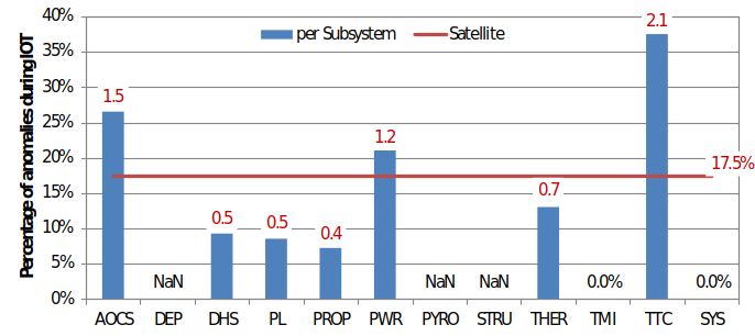
Fig. 9.4.34 Percentage of major anomalies that were observed during In-Orbit Testing at satellite level (red line) and for the different subsystems (bar chart) – given as an example#
Classification by root cause and severity
As discussed in Section 9.4.9.2, systematic failures and anomalies can be further classified by the detailed root cause, from design and manufacturing errors to operations. Fig. 9.4.35 shows the classification of observed anomalies by root cause, using the definitions from the data source, as outlined in Section 9.4.9.3.1. The repartition by severity category clearly shows that anomalies leading to hardware failures and/or having an impact on the mission (severity 1 to 4) are mainly due to root causes in hardware design or manufacturing. Severe events due to other root causes are rare exceptions, as can be seen also from Fig. 9.4.36.
Note
Hardware failure” is here defined in a wide sense, i.e. all anomalies having an impact on the mission (severity 1 to 3) are considered as failures, even though they cannot involve a definitive hardware failure.
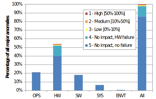
Fig. 9.4.35 Classification of major anomalies by severity category and root cause (Operations OPS, hardware design/manufacturing hardware, software error SW, system design/manufacturing SYS, Environmental design ENVT)#
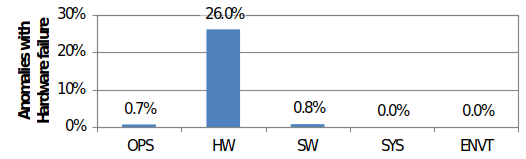
Fig. 9.4.36 Percentage of anomalies with hardware failure (severity category 1 to 4) for the different root causes (see Fig. 9.4.35 for definitions). The percentage in this figure relates to the total number of major anomalies (with or without Hardware failure) attributed to a specific root cause.#
Classification by technical domain (EEE, mechanical, miscellaneous)
The repartition by satellite subsystem already gives a first indication on the relevance of systematic anomalies related to EEE, mechanical or miscellaneous items. For the anomalies whose root cause is classified as “hardware”, Fig. 9.4.37 gives further information on the repartition by the type of the equipment involved, and by the details of the root cause (design or manufacturing error). The classification is done at equipment level, considering all satellite subsystems and using the same three classes as outlined in Part 3 - EEE, Part 4 - MEC and Part 5 - MIS
It can be seen that the contribution of “mechanical” anomalies is very low, which can be explained by the fact that many of the most error-prone satellite elements are classified as “miscellaneous items” in this handbook.
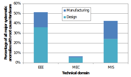
Fig. 9.4.37 Repartition of anomalies whose root cause is classified as “hardware” by the type of the equipment (EEE, mechanical – MEC, miscellaneous – MIS) involved and the detailed root cause#