(syst_annex_a=)

9.5. Annex A: Modelling results

As discussed in Section 9.4.9.3.2, the modelling provides an anomaly occurrence model at satellite level and a set of conditional probabilities for the repartition of anomalies by subsystem and severity. Results and parameters for each model component are given in the following, based on the data set described in Section 9.4.9.3.1 and under the assumptions and limitations discussed above.

9.5.1. Anomaly occurrence model

The data base used for the estimation of the parameters is illustrated in Fig. 9.5.1. The portfolio of satellites is almost equally distributed over the time which indicates that the number of launches in each year does not vary too much in the considered time. Per satellite, an anomaly can occur several times within one satellite (repeated events). The total number of anomalies is thus larger than the number of satellites in the portfolio.

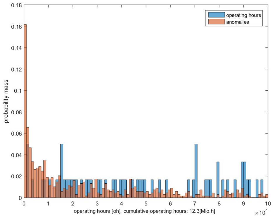
Fig. 9.5.1 Database for modelling the time dependent anomaly occurrence rate

The rate of anomaly occurrence (all severities) derived from the Poisson/Weibull model fitted to the data is shown inFig. 9.5.2. Markov Chain Monte Carlo simulations were used to determine the posterior distribution of the model parameters \(\alpha\) and \(\beta\). As can be seen from the 90% confidence interval, the statistical uncertainty associated with the model is rather small due to the fact that also minor anomalies are considered in the data sample, leading to a considerable sample size.

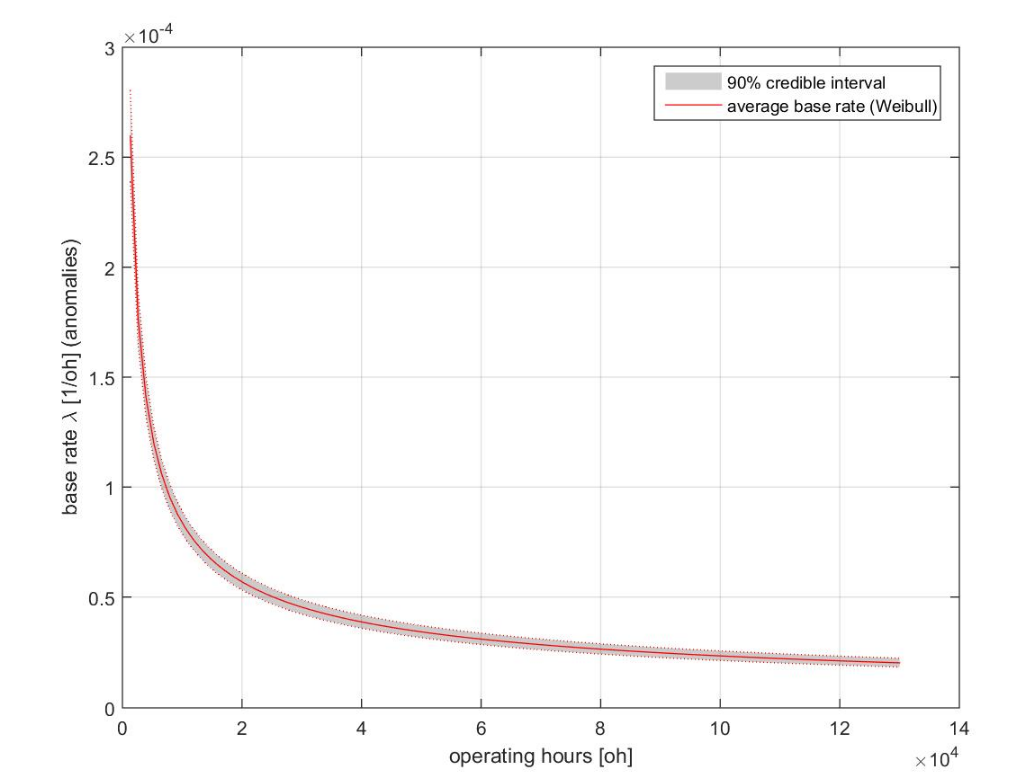
Fig. 9.5.2 Time dependent anomaly occurrence rate due to systematic root causes based on the Poisson/Weibull model for anomalies observed at satellite level (all severities)

The bivariate distribution of the model parameters after convergence of the MCMC simulation is illustrated in Fig. 9.5.3. It can be seen that the shape parameter of the Weibull model is clearly below unity, implying a decreasing failure rate as shown in Fig. 9.5.2.

The parameters of the Weibull distribution are highly correlated. This correlation needs to be considered when calculating the failure rate. The joint distribution of the Weibull parameters can be approximated here by a bivariate normal distribution.

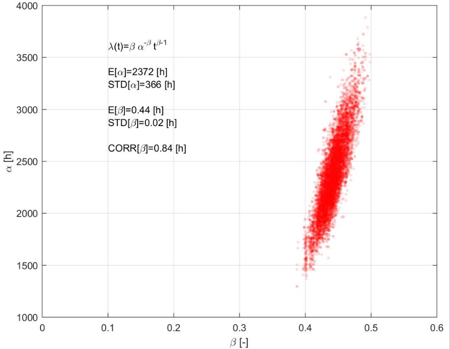
Fig. 9.5.3 Posterior distribution of the model parameters for the Poisson/Weibull anomaly occurrence model, based on the MCMC chains [10’000 post burn in simulations]

Table 9.5.1 Posterior parameters of the Weibull distribution for the occurrence rate of anomalies

Parameter	Mean (posterior)	Std (posterior)	cov	Correlation
\(\alpha'' [\text{h}]\)	0.44	0.02	0.05	0.84
\(\beta'' [-]\)	2372	366	0.15	0.84

9.5.2. Anomaly repartition by subsystem

The posterior marginal probabilities for the repartition of the anomalies by subsystem is provided in Fig. 9.5.4. The marginal probability distributions follow beta distribution. Samples from the multivariate probability distribution are correlated and can be generated by using the parameters of the Dirichlet distribution provided in Table 9.5.2.

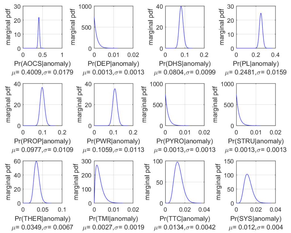
Fig. 9.5.4 Posterior marginal distributions of the conditional probabilities for the repartition of anomalies by subsystem

These probabilities can be combined with the overall anomaly occurrence rate. As mentioned before, the resulting distribution of subsystem anomalies over time is questionable due to the assumption that the shape of the curve is the same for all subsystems.

Table 9.5.2 Posterior parameters of the Dirichlet distribution for the repartition of anomalies by subsystem

Parameter	\(\eta_{i}''\) (posterior)
AOCS	299
DEP	1
DHS	60
PL	185
PROP	73
PWR	79
PYRO	1
STRU	1
THER	26
TMI	2
TTC	10
SYS	9

9.5.3. Anomaly repartition by hardware failure

Based on the model provided in Section 9.4.9.3.2, the marginal posterior probability of hardware failure conditional on an anomaly is shown in Fig. 9.5.5. The parameters of the Dirichlet distribution are given in Table 9.5.2 (satellite level).

Since the model is a bivariate Dirichlet distribution the two outcomes are fully negatively correlated and can thus be fully represented by a 2-parameter beta distribution.

The marginal posterior probability of hardware failure conditional on an anomaly for all subsystems can be sampled from the Dirichlet distribution using the parameters provided in Table 9.5.2. The corresponding marginal posterior distributions for all subsystems are provided in Fig. 9.5.6.

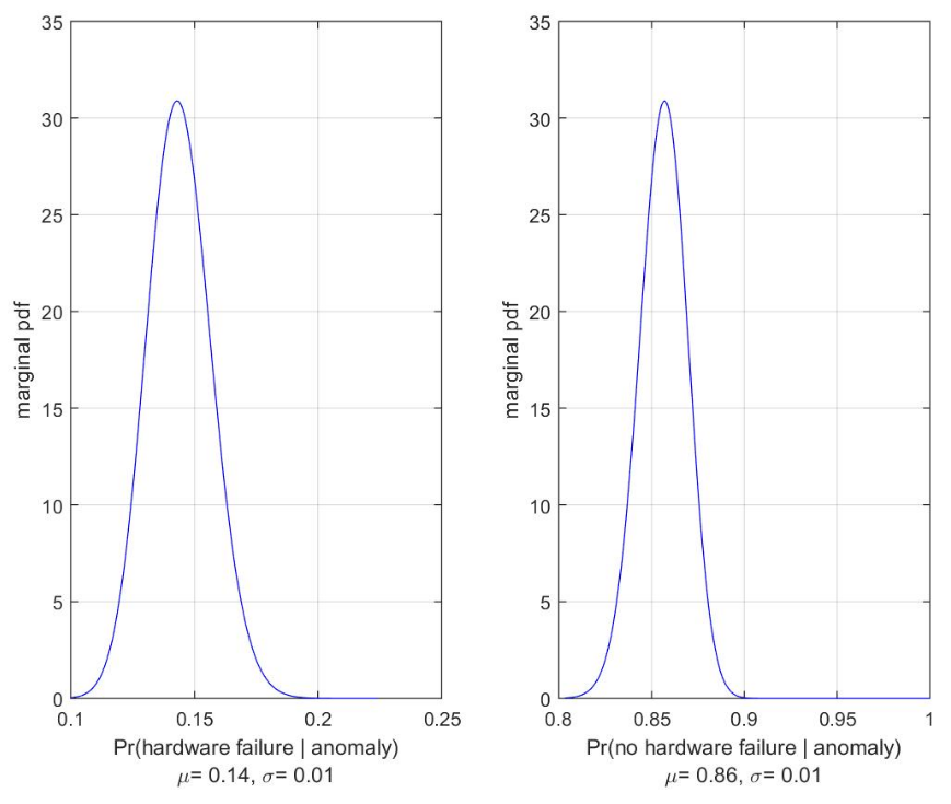
Fig. 9.5.5 Posterior marginal distributions of the conditional probabilities for the repartition of anomalies by hardware failures on satellite level.

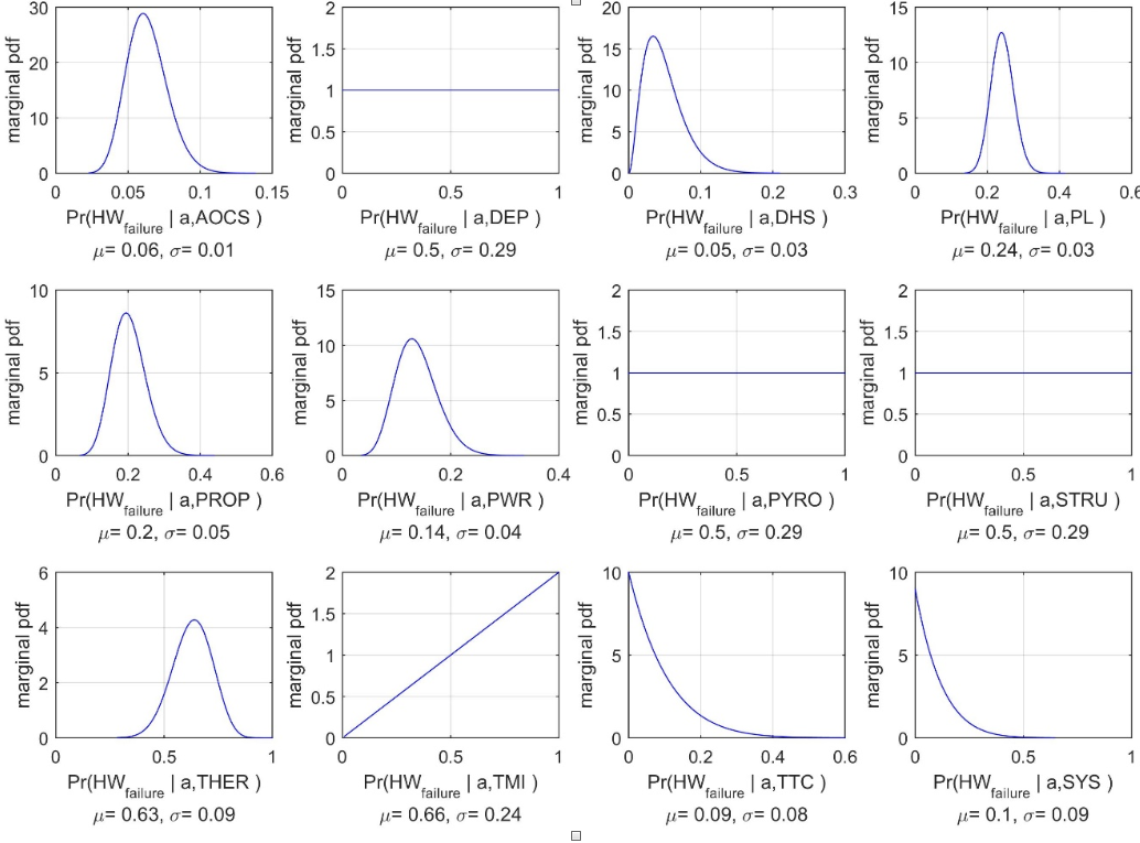
Fig. 9.5.6 Posterior marginal distributions of the conditional probabilities for the repartition of anomalies for the subsystems(a=anomaly ).

Table 9.5.3 Posterior parameters of the Dirichlet distribution for the repartition of a hardware failure for given an anomaly for on satellite level and for all subsystems

Parameter	\(\delta_{1}''\,[h]\) (posterior)	\(\delta_{2}''\,[-]\) (posterior)
Satellite level	106	630
AOCS	19	281
DEP	1	1
DHS	3	58
PL	45	141
PROP	15	59
PWR	11	69
PYRO	1	1
STRU	1	1
THER	17	10
TMI	2	1
TTC	1	10
SYS	1	1

9.5.4. Anomaly repartition by severity given hardware failure

The repartition of anomalies by severity category is modelled with the following set of conditional probabilities fitted to the data.

The marginal distributions of the four probabilities, representing statistical uncertainty due to the limited sample size used for modelling, are shown in Fig. 9.5.7.

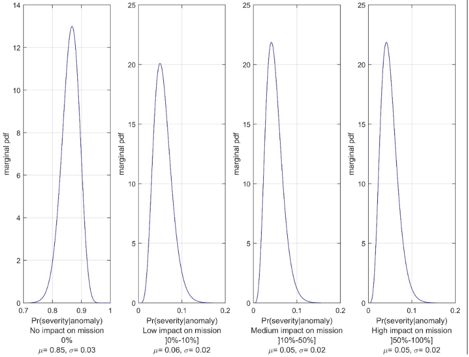
Fig. 9.5.7 Posterior marginal distributions of the conditional probabilities for the repartition of anomalies by severity considered at satellite level

The probabilities provided in Fig. 9.5.7 are conditional on anomaly occurrence (Table 9.5.1) and on hardware failure (Table 9.5.3 for satellite level). When combined with the anomaly occurrence model, time-dependent occurrence rates can be derived for the different severity categories, as illustrated in Fig. 9.5.8 below (the 90% confidence interval now includes the uncertainty inherent in the anomaly repartition model and the hardware failure model).

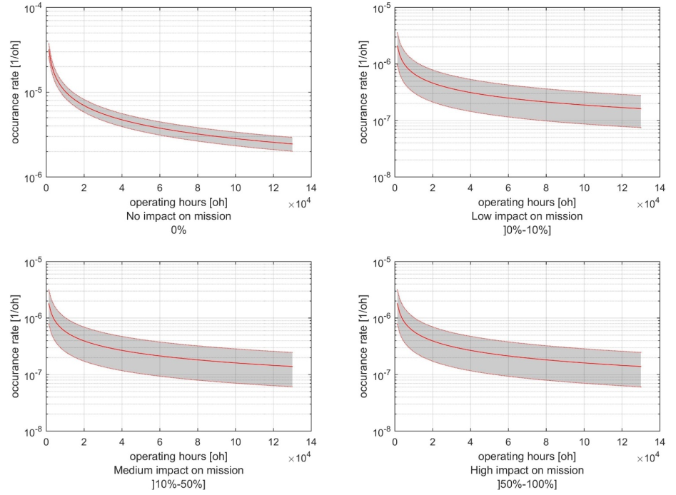
Fig. 9.5.8 Anomaly occurrence rate for different severity categories, considered at satellite level

The posterior parameters of the Dirichlet distribution for the different severity classes conditional on an anomaly and a hardware failure for satellite level and for all subsystems Table 9.5.3.

Table 9.5.4 Posterior parameters of the Dirichlet distribution for the different severity classes conditional on an anomaly and a hardware failure at satellite level and for all subsystems

Parameter	\(\theta_{1}'' [h]\) High impact	\(\theta_{2}'' [h]\) Medium impact	\(\theta_{3}'' [h]\) Low impact	\(\theta_{4}'' [-]\) No impact
Satellite level	6	6	7	90
AOCS	3	2	2	15
DEP	1	1	1	1
DHS	1	1	1	3
PL	1	1	3	43
PROP	2	1	1	14
PWR	3	5	2	4
PYRO	1	1	1	1
STRU	1	1	1	1
THER	1	1	1	1
TMI	1	1	2	16
TTC	1	1	2	1
SYS	1	1	1	1